3 Simple iteration
Processing multiple files that contain different parts of the same dataset
This chapter introduces iteration as a concept to repeat the same operation over a sequence of inputs. It is largely independent of the previous chapter.
The following packages are required throughout this chapter:
library(tidyverse)
library(here)
3.1 Vectors and columns
So far we focus on the data frame, or tibble, as primary object for data analysis. Internally, a tibble is a list of vectors of the same length. Accessing a row in a tibble requires finding the same index in that list of vectors.
Here we explore the relationship between columns of data frames and their corresponding vectors, i.e. the answer to “how to get from one to the other?”:
We can e.g. get a vector with the files in a specific directory of our current project2 like this:
files <- dir(here("data/weather"), full.names = TRUE)
files
## [1] "/home/travis/build/krlmlr/tidyprog/data/weather/berlin.xlsx"
## [2] "/home/travis/build/krlmlr/tidyprog/data/weather/tel_aviv.xlsx"
## [3] "/home/travis/build/krlmlr/tidyprog/data/weather/toronto.xlsx"
## [4] "/home/travis/build/krlmlr/tidyprog/data/weather/zurich.xlsx"You can create a tibble from it using tibble::enframe():
files_df <-
  files %>%
  enframe()

files_df
## # A tibble: 4 x 2
## name value
## <int> <chr>
## 1 1 /home/travis/build/krlmlr/tidyprog/data/weather/berlin.xlsx
## 2 2 /home/travis/build/krlmlr/tidyprog/data/weather/tel_aviv.xlsx
## 3 3 /home/travis/build/krlmlr/tidyprog/data/weather/toronto.xlsx
## 4 4 /home/travis/build/krlmlr/tidyprog/data/weather/zurich.xlsx
The name column might be unwanted in some cases. Suppress its creation by setting name = NULL:
files_df_1 <-
  files %>%
  enframe(name = NULL)

files_df_1
## # A tibble: 4 x 1
## value
## <chr>
## 1 /home/travis/build/krlmlr/tidyprog/data/weather/berlin.xlsx
## 2 /home/travis/build/krlmlr/tidyprog/data/weather/tel_aviv.xlsx
## 3 /home/travis/build/krlmlr/tidyprog/data/weather/toronto.xlsx
## 4 /home/travis/build/krlmlr/tidyprog/data/weather/zurich.xlsx
Another way to create a tibble from a vector is using tibble::tibble().
You can name the newly created columns by assigning the vectors they are created from to (quoted or unquoted) column names:
tibble(filename = files)## # A tibble: 4 x 1
## filename
## <chr>
## 1 /home/travis/build/krlmlr/tidyprog/data/weather/berlin.xlsx
## 2 /home/travis/build/krlmlr/tidyprog/data/weather/tel_aviv.xlsx
## 3 /home/travis/build/krlmlr/tidyprog/data/weather/toronto.xlsx
## 4 /home/travis/build/krlmlr/tidyprog/data/weather/zurich.xlsx
The other direction – producing a vector from a tibble column – works with dplyr::pull().
By default pull() will turn the rightmost column into a vector and ignore the rest of the tibble:
files_df %>%
  pull()
## [1] "/home/travis/build/krlmlr/tidyprog/data/weather/berlin.xlsx"
## [2] "/home/travis/build/krlmlr/tidyprog/data/weather/tel_aviv.xlsx"
## [3] "/home/travis/build/krlmlr/tidyprog/data/weather/toronto.xlsx"
## [4] "/home/travis/build/krlmlr/tidyprog/data/weather/zurich.xlsx"Turn a specific column into a vector by providing the desired column name to pull(), either quoted or unquoted:
files_df %>%
  pull(name)
## [1] 1 2 3 43.1.1 Exercises
Investigate the output of
fs::dir_ls()withenframe(). Explain.# install.packages("fs") fs::dir_ls() fs::dir_ls() %>% ___()## # A tibble: 45 x 2 ## name value ## <chr> <fs::path> ## 1 1.Rmd 1.Rmd ## 2 12-intro.Rmd 12-intro.Rmd ## 3 2.Rmd 2.Rmd ## # … with 42 more rows
3.2 Named vectors and two-column tibbles
Click here to show setup code.
library(tidyverse)
library(here)
Here we look at tidyverse-functions to work with named vectors and tibbles with more columns and the relations netween the two.
As seen in section “Data”, load a table – here a dictionary detailing information related to an id-like name – from an MS Excel file with readxl::read_excel():
dict <- readxl::read_excel(here("data/cities.xlsx"))
dict
## # A tibble: 4 x 5
## city_code weather_filename name lng lat
## <chr> <chr> <chr> <dbl> <dbl>
## 1 berlin data/weather/berlin.xlsx Berlin 13.4 52.5
## 2 toronto data/weather/toronto.xlsx Toronto -79.4 43.7
## 3 tel_aviv data/weather/tel_aviv.xlsx Tel Aviv 34.8 32.1
## 4 zurich data/weather/zurich.xlsx Zürich 8.54 47.4
Use pull() as seen in the last chapter:
dict %>%
  pull(weather_filename)
## [1] "data/weather/berlin.xlsx" "data/weather/toronto.xlsx"
## [3] "data/weather/tel_aviv.xlsx" "data/weather/zurich.xlsx"Create absolute paths using here::here():
dict %>%
  pull(weather_filename) %>%
  here()
## [1] "/home/travis/build/krlmlr/tidyprog/data/weather/berlin.xlsx"
## [2] "/home/travis/build/krlmlr/tidyprog/data/weather/toronto.xlsx"
## [3] "/home/travis/build/krlmlr/tidyprog/data/weather/tel_aviv.xlsx"
## [4] "/home/travis/build/krlmlr/tidyprog/data/weather/zurich.xlsx"Produce a named vector with tibble::deframe(), which is thought as the inverse function to enframe().
When given a 2-column tibble, deframe() will by default use the first column for the names and the second column for the values of the resulting vector.
When given a 1-column tibble, it creates an unnamed vector.
When given a more-than-2-column tibble, it will use the first two columns as name- and value-columns for the resulting vector, ignore the rest and in addition give a warning that it expects a one- or two-column data frame.
weather_filenames <-
  dict %>%
  select(city_code, weather_filename) %>%
  deframe()
weather_filenames
## berlin toronto
## "data/weather/berlin.xlsx" "data/weather/toronto.xlsx"
## tel_aviv zurich
## "data/weather/tel_aviv.xlsx" "data/weather/zurich.xlsx"The names() function accesses the names of a vector:
weather_filenames %>%
  names()
## [1] "berlin" "toronto" "tel_aviv" "zurich"Some operations producing vectors from vectors cause the names to be lost:
paste0("'", weather_filenames, "'")## [1] "'data/weather/berlin.xlsx'" "'data/weather/toronto.xlsx'"
## [3] "'data/weather/tel_aviv.xlsx'" "'data/weather/zurich.xlsx'"weather_filenames %>%
here()## [1] "/home/travis/build/krlmlr/tidyprog/data/weather/berlin.xlsx"
## [2] "/home/travis/build/krlmlr/tidyprog/data/weather/toronto.xlsx"
## [3] "/home/travis/build/krlmlr/tidyprog/data/weather/tel_aviv.xlsx"
## [4] "/home/travis/build/krlmlr/tidyprog/data/weather/zurich.xlsx"A possible solution can be in many cases to change the order of the transformations, so that the creation of the named vector comes last (or at least later):
dict %>%
  mutate(weather_filename_here = here(weather_filename))
## # A tibble: 4 x 6
## city_code weather_filename name lng lat weather_filename_here
## <chr> <chr> <chr> <dbl> <dbl> <chr>
## 1 berlin data/weather/berl… Berlin 13.4 52.5 /home/travis/build/krlm…
## 2 toronto data/weather/toro… Toron… -79.4 43.7 /home/travis/build/krlm…
## 3 tel_aviv data/weather/tel_… Tel A… 34.8 32.1 /home/travis/build/krlm…
## 4 zurich data/weather/zuri… Zürich 8.54 47.4 /home/travis/build/krlm…
dict %>%
  mutate(weather_filename_here = here(weather_filename)) %>%
  select(city_code, weather_filename_here)
## # A tibble: 4 x 2
## city_code weather_filename_here
## <chr> <chr>
## 1 berlin /home/travis/build/krlmlr/tidyprog/data/weather/berlin.xlsx
## 2 toronto /home/travis/build/krlmlr/tidyprog/data/weather/toronto.xlsx
## 3 tel_aviv /home/travis/build/krlmlr/tidyprog/data/weather/tel_aviv.xlsx
## 4 zurich /home/travis/build/krlmlr/tidyprog/data/weather/zurich.xlsx
dict %>%
  mutate(weather_filename_here = here(weather_filename)) %>%
  select(city_code, weather_filename_here) %>%
  deframe()
## berlin
## "/home/travis/build/krlmlr/tidyprog/data/weather/berlin.xlsx"
## toronto
## "/home/travis/build/krlmlr/tidyprog/data/weather/toronto.xlsx"
## tel_aviv
## "/home/travis/build/krlmlr/tidyprog/data/weather/tel_aviv.xlsx"
## zurich
## "/home/travis/build/krlmlr/tidyprog/data/weather/zurich.xlsx"3.2.1 Exercises
Obtain a mapping between city code and city name as a named vector.
dict %>%
  select(___, ___) %>%
  deframe()
## berlin toronto tel_aviv zurich ## "Berlin" "Toronto" "Tel Aviv" "Zürich"Convert the output of
fs::dir_info()to that seen fromfs::dir_ls(). How do you make sure that the vector is named?# install.packages("fs") fs::dir_info() fs::dir_info() %>% pull(___) fs::dir_info() %>% select(_____, _____) %>% ___()## # A tibble: 45 x 18 ## path type size permissions modification_time user group ## <fs::path> <fct> <fs::b> <fs::perms> <dttm> <chr> <chr> ## 1 1.Rmd file 56 rw-rw-r-- 2019-05-29 19:54:06 trav… trav… ## 2 12-intro.… file 5.85K rw-rw-r-- 2019-05-29 19:54:06 trav… trav… ## 3 2.Rmd file 370 rw-rw-r-- 2019-05-29 19:54:06 trav… trav… ## # … with 42 more rows, and 11 more variables: device_id <dbl>, ## # hard_links <dbl>, special_device_id <dbl>, inode <dbl>, ## # block_size <dbl>, blocks <dbl>, flags <int>, generation <dbl>, ## # access_time <dttm>, change_time <dttm>, birth_time <dttm>## 1.Rmd 12-intro.Rmd 2.Rmd ## 21-function.Rmd 22-args.Rmd 23-intermediate.Rmd ## 24-args-default.Rmd 25-args-multi.Rmd 26-args-matching.Rmd ## 3.Rmd 31-dir.Rmd 32-names.Rmd ## 33-index.Rmd 34-construct.Rmd 35-map.Rmd ## 36-map-manip.Rmd 37-map-type.Rmd 4.Rmd ## 41-map2.Rmd 42-mutate-map.Rmd## 1.Rmd 12-intro.Rmd 2.Rmd ## 21-function.Rmd 22-args.Rmd 23-intermediate.Rmd ## 24-args-default.Rmd 25-args-multi.Rmd 26-args-matching.Rmd ## 3.Rmd 31-dir.Rmd 32-names.Rmd ## 33-index.Rmd 34-construct.Rmd 35-map.Rmd ## 36-map-manip.Rmd 37-map-type.Rmd 4.Rmd ## 41-map2.Rmd 42-mutate-map.Rmd
3.3 Indexing/subsetting
Click here to show setup code.
library(tidyverse)
library(here)

dict <- readxl::read_excel(here("data/cities.xlsx"))
Here we look at the indexing of a named vector (works equivalently for a named list).
We start with the data frame dict from section “Named vectors and two-column tibbles”.
Create named vector of the – future – input files:
input_files <-
  dict %>%
  select(city_code, weather_filename) %>%
  deframe()
input_files
## berlin toronto
## "data/weather/berlin.xlsx" "data/weather/toronto.xlsx"
## tel_aviv zurich
## "data/weather/tel_aviv.xlsx" "data/weather/zurich.xlsx"names(input_files)## [1] "berlin" "toronto" "tel_aviv" "zurich"There are different ways of accessing individual entries of the named vector:
input_files[1]## berlin
## "data/weather/berlin.xlsx"input_files[[1]]## [1] "data/weather/berlin.xlsx"input_files["berlin"]## berlin
## "data/weather/berlin.xlsx"input_files[["berlin"]]## [1] "data/weather/berlin.xlsx"Choose multiple entries with:
input_files[1:2]## berlin toronto
## "data/weather/berlin.xlsx" "data/weather/toronto.xlsx"input_files[c("berlin", "zurich")]## berlin zurich
## "data/weather/berlin.xlsx" "data/weather/zurich.xlsx"Consistent pipe-friendly access of single elements:
input_files %>%
  pluck(1)
## [1] "data/weather/berlin.xlsx"input_files %>%
pluck("berlin")## [1] "data/weather/berlin.xlsx"3.3.1 Exercises
Explain the difference between
[and[[subsetting.Implement a variant of subsetting in “tibble-land” with a combination of
enframe(),slice()orfilter(), anddeframe():input_files %>% enframe() %>% ___(_____) %>% deframe()## toronto ## "data/weather/toronto.xlsx"
3.4 Construction
Click here to show setup code.
The c() function constructs vectors.
All elements of a vector must have the same type.
c(1, 2, 3)## [1] 1 2 3c(1:3, 5)## [1] 1 2 3 5c(1:3, "5")## [1] "1" "2" "3" "5"Lists are constructed with list().
They are a special type of vector – they can contain elements of different type and length.
list(1, 2, 3)## [[1]]
## [1] 1
##
## [[2]]
## [1] 2
##
## [[3]]
## [1] 3list(1:3, 5)## [[1]]
## [1] 1 2 3
##
## [[2]]
## [1] 5list(1:3, "5")## [[1]]
## [1] 1 2 3
##
## [[2]]
## [1] "5"Lists can also contain other lists.
nested <- list(
  1:3,
  list(4, "5"),
  list(
    list(letters[6:8]),
    9
  )
)

nested
## [[1]]
## [1] 1 2 3
##
## [[2]]
## [[2]][[1]]
## [1] 4
##
## [[2]][[2]]
## [1] "5"
##
##
## [[3]]
## [[3]][[1]]
## [[3]][[1]][[1]]
## [1] "f" "g" "h"
##
##
## [[3]][[2]]
## [1] 9str(nested)## List of 3
## $ : int [1:3] 1 2 3
## $ :List of 2
## ..$ : num 4
## ..$ : chr "5"
## $ :List of 2
## ..$ :List of 1
## .. ..$ : chr [1:3] "f" "g" "h"
## ..$ : num 9Vectors (and also lists) can have names.
c(a = 1, b = 2, c = 3)## a b c
## 1 2 3list(a = 1:3, b = 5)## $a
## [1] 1 2 3
##
## $b
## [1] 5rlang::set_names(1:3, letters[1:3])## a b c
## 1 2 3The new {vctrs} package defines a data type for lists where all elements have the same type: a stricter list, but more powerful than a bare vector.
#vctrs::list_of(1, 2, 3)
#try(vctrs::list_of(1, 2, "3"))
#vctrs::list_of(letters[1:3], "e")
3.4.1 Exercises
Explain the differences between the outputs below.
c(a = list(1:3), b = list(4:5))## $a ## [1] 1 2 3 ## ## $b ## [1] 4 5list(a = list(1:3), b = list(4:5))## $a ## $a[[1]] ## [1] 1 2 3 ## ## ## $b ## $b[[1]] ## [1] 4 5
3.5 Processing multiple files
Click here to show setup code.
library(tidyverse)
library(here)

dict <- readxl::read_excel(here("data/cities.xlsx"))

input_files <-
  dict %>%
  select(city_code, weather_filename) %>%
  deframe()
Here we look at how to act on each entry of a list or a vector using purrr::map():
We start with the named vector input_files from section “Indexing”.
As just seen, manually choosing just one entry of a vector works like so:
input_files[[1]]## [1] "data/weather/berlin.xlsx"here(input_files[[1]])## [1] "/home/travis/build/krlmlr/tidyprog/data/weather/berlin.xlsx"readxl::read_excel(here(input_files[[1]]))## # A tibble: 49 x 18
## time summary icon precipIntensity precipProbabili…
## <dttm> <chr> <chr> <dbl> <dbl>
## 1 2019-04-28 15:00:00 Mostly… part… 0 0
## 2 2019-04-28 16:00:00 Mostly… part… 0 0
## 3 2019-04-28 17:00:00 Mostly… part… 0 0
## # … with 46 more rows, and 13 more variables: temperature <dbl>,
## # apparentTemperature <dbl>, dewPoint <dbl>, humidity <dbl>,
## # pressure <dbl>, windSpeed <dbl>, windGust <dbl>, windBearing <dbl>,
## # cloudCover <dbl>, uvIndex <dbl>, visibility <dbl>, ozone <dbl>,
## # precipType <chr>
However, if we try to read all files from the vector with read_excel(), this fails:
here(input_files)## [1] "/home/travis/build/krlmlr/tidyprog/data/weather/berlin.xlsx"
## [2] "/home/travis/build/krlmlr/tidyprog/data/weather/toronto.xlsx"
## [3] "/home/travis/build/krlmlr/tidyprog/data/weather/tel_aviv.xlsx"
## [4] "/home/travis/build/krlmlr/tidyprog/data/weather/zurich.xlsx"try(readxl::read_excel(here(input_files)))## Error : `path` must be a stringUnlike here(), the read_excel() function can process only one file at a time.
We need to iterate explicitly.
With map(), you can successively work through the whole vector and each time let the same function deal with the respective entry.
The output of map() is a list where each element contains one results.
The list is named if the input is named:
input_data <-
map(input_files, ~ readxl::read_excel(here(.)))The map() call above is equivalent to the following code:
input_data <-
list(
berlin = readxl::read_excel(here(input_files[[1]])),
toronto = readxl::read_excel(here(input_files[[2]])),
tel_aviv = readxl::read_excel(here(input_files[[3]])),
zurich = readxl::read_excel(here(input_files[[4]]))
)Let’s take a closer look at what we produced:
input_data## $berlin
## # A tibble: 49 x 18
##   time                summary icon  precipIntensity precipProbabili…
##   <dttm>              <chr>   <chr>           <dbl>            <dbl>
## 1 2019-04-28 15:00:00 Mostly… part…               0                0
## 2 2019-04-28 16:00:00 Mostly… part…               0                0
## 3 2019-04-28 17:00:00 Mostly… part…               0                0
## # … with 46 more rows, and 13 more variables: temperature <dbl>,
## #   apparentTemperature <dbl>, dewPoint <dbl>, humidity <dbl>,
## #   pressure <dbl>, windSpeed <dbl>, windGust <dbl>, windBearing <dbl>,
## #   cloudCover <dbl>, uvIndex <dbl>, visibility <dbl>, ozone <dbl>,
## #   precipType <chr>
##
## $toronto
## # A tibble: 49 x 18
## time summary icon precipIntensity precipProbabili…
## <dttm> <chr> <chr> <dbl> <dbl>
## 1 2019-04-28 15:00:00 Partly… part… 0 0
## 2 2019-04-28 16:00:00 Clear clea… 0 0
## 3 2019-04-28 17:00:00 Clear clea… 0 0
## # … with 46 more rows, and 13 more variables: temperature <dbl>,
## # apparentTemperature <dbl>, dewPoint <dbl>, humidity <dbl>,
## # pressure <dbl>, windSpeed <dbl>, windGust <dbl>, windBearing <dbl>,
## # cloudCover <dbl>, uvIndex <dbl>, visibility <dbl>, ozone <dbl>,
## # precipType <chr>
##
## $tel_aviv
## # A tibble: 49 x 17
## time summary icon precipIntensity precipProbabili…
## <dttm> <chr> <chr> <dbl> <dbl>
## 1 2019-04-28 15:00:00 Partly… part… 0 0
## 2 2019-04-28 16:00:00 Clear clea… 0 0
## 3 2019-04-28 17:00:00 Clear clea… 0 0
## # … with 46 more rows, and 12 more variables: temperature <dbl>,
## # apparentTemperature <dbl>, dewPoint <dbl>, humidity <dbl>,
## # pressure <dbl>, windSpeed <dbl>, windGust <dbl>, windBearing <dbl>,
## # cloudCover <dbl>, uvIndex <dbl>, visibility <dbl>, ozone <dbl>
##
## $zurich
## # A tibble: 49 x 18
## time summary icon precipIntensity precipProbabili…
## <dttm> <chr> <chr> <dbl> <dbl>
## 1 2019-04-28 15:00:00 Mostly… part… 0.267 0.28
## 2 2019-04-28 16:00:00 Mostly… part… 0.198 0.27
## 3 2019-04-28 17:00:00 Mostly… part… 0.137 0.25
## # … with 46 more rows, and 13 more variables: precipType <chr>,
## # temperature <dbl>, apparentTemperature <dbl>, dewPoint <dbl>,
## # humidity <dbl>, pressure <dbl>, windSpeed <dbl>, windGust <dbl>,
## # windBearing <dbl>, cloudCover <dbl>, uvIndex <dbl>, visibility <dbl>,
## # ozone <dbl>
input_data[[1]]## # A tibble: 49 x 18
## time summary icon precipIntensity precipProbabili…
## <dttm> <chr> <chr> <dbl> <dbl>
## 1 2019-04-28 15:00:00 Mostly… part… 0 0
## 2 2019-04-28 16:00:00 Mostly… part… 0 0
## 3 2019-04-28 17:00:00 Mostly… part… 0 0
## # … with 46 more rows, and 13 more variables: temperature <dbl>,
## # apparentTemperature <dbl>, dewPoint <dbl>, humidity <dbl>,
## # pressure <dbl>, windSpeed <dbl>, windGust <dbl>, windBearing <dbl>,
## # cloudCover <dbl>, uvIndex <dbl>, visibility <dbl>, ozone <dbl>,
## # precipType <chr>
names(input_data)## [1] "berlin" "toronto" "tel_aviv" "zurich"map() can be included in your pipe in the following way:
input_files %>%
map(~ readxl::read_excel(here(.)))## $berlin
## # A tibble: 49 x 18
##   time                summary icon  precipIntensity precipProbabili…
##   <dttm>              <chr>   <chr>           <dbl>            <dbl>
## 1 2019-04-28 15:00:00 Mostly… part…               0                0
## 2 2019-04-28 16:00:00 Mostly… part…               0                0
## 3 2019-04-28 17:00:00 Mostly… part…               0                0
## # … with 46 more rows, and 13 more variables: temperature <dbl>,
## #   apparentTemperature <dbl>, dewPoint <dbl>, humidity <dbl>,
## #   pressure <dbl>, windSpeed <dbl>, windGust <dbl>, windBearing <dbl>,
## #   cloudCover <dbl>, uvIndex <dbl>, visibility <dbl>, ozone <dbl>,
## #   precipType <chr>
##
## $toronto
 ## # A tibble: 49 x 18
 ##   time                summary icon  precipIntensity precipProbabili…
 ##   <dttm>              <chr>   <chr>           <dbl>            <dbl>
 ## 1 2019-04-28 15:00:00 Partly… part…               0                0
 ## 2 2019-04-28 16:00:00 Clear   clea…               0                0
 ## 3 2019-04-28 17:00:00 Clear   clea…               0                0
 ## # … with 46 more rows, and 13 more variables: temperature <dbl>,
 ## #   apparentTemperature <dbl>, dewPoint <dbl>, humidity <dbl>,
 ## #   pressure <dbl>, windSpeed <dbl>, windGust <dbl>, windBearing <dbl>,
 ## #   cloudCover <dbl>, uvIndex <dbl>, visibility <dbl>, ozone <dbl>,
 ## #   precipType <chr>
 ##
 ## $tel_aviv
 ## # A tibble: 49 x 17
 ##   time                summary icon  precipIntensity precipProbabili…
 ##   <dttm>              <chr>   <chr>           <dbl>            <dbl>
 ## 1 2019-04-28 15:00:00 Partly… part…               0                0
 ## 2 2019-04-28 16:00:00 Clear   clea…               0                0
 ## 3 2019-04-28 17:00:00 Clear   clea…               0                0
 ## # … with 46 more rows, and 12 more variables: temperature <dbl>,
 ## #   apparentTemperature <dbl>, dewPoint <dbl>, humidity <dbl>,
 ## #   pressure <dbl>, windSpeed <dbl>, windGust <dbl>, windBearing <dbl>,
 ## #   cloudCover <dbl>, uvIndex <dbl>, visibility <dbl>, ozone <dbl>
##
## $zurich
## # A tibble: 49 x 18
## time summary icon precipIntensity precipProbabili…
## <dttm> <chr> <chr> <dbl> <dbl>
## 1 2019-04-28 15:00:00 Mostly… part… 0.267 0.28
## 2 2019-04-28 16:00:00 Mostly… part… 0.198 0.27
## 3 2019-04-28 17:00:00 Mostly… part… 0.137 0.25
## # … with 46 more rows, and 13 more variables: precipType <chr>,
## # temperature <dbl>, apparentTemperature <dbl>, dewPoint <dbl>,
## # humidity <dbl>, pressure <dbl>, windSpeed <dbl>, windGust <dbl>,
## # windBearing <dbl>, cloudCover <dbl>, uvIndex <dbl>, visibility <dbl>,
## # ozone <dbl>
3.5.1 Exercises
Read only the data for Toronto and Tel Aviv, using subsetting or
filter(). Compare.input_files[_____] %>% map(~ readxl::read_excel(here(.))) input_files %>% ___() %>% filter(name %in% c(_____)) %>% ___() %>% map(~ readxl::read_excel(here(.)))## $toronto ## # A tibble: 49 x 18 ## time summary icon precipIntensity precipProbabili… ## <dttm> <chr> <chr> <dbl> <dbl> ## 1 2019-04-28 15:00:00 Partly… part… 0 0 ## 2 2019-04-28 16:00:00 Clear clea… 0 0 ## 3 2019-04-28 17:00:00 Clear clea… 0 0 ## # … with 46 more rows, and 13 more variables: temperature <dbl>, ## # apparentTemperature <dbl>, dewPoint <dbl>, humidity <dbl>, ## # pressure <dbl>, windSpeed <dbl>, windGust <dbl>, windBearing <dbl>, ## # cloudCover <dbl>, uvIndex <dbl>, visibility <dbl>, ozone <dbl>, ## # precipType <chr> ## ## $tel_aviv ## # A tibble: 49 x 17 ## time summary icon precipIntensity precipProbabili… ## <dttm> <chr> <chr> <dbl> <dbl> ## 1 2019-04-28 15:00:00 Partly… part… 0 0 ## 2 2019-04-28 16:00:00 Clear clea… 0 0 ## 3 2019-04-28 17:00:00 Clear clea… 0 0 ## # … with 46 more rows, and 12 more variables: temperature <dbl>, ## # apparentTemperature <dbl>, dewPoint <dbl>, humidity <dbl>, ## # pressure <dbl>, windSpeed <dbl>, windGust <dbl>, windBearing <dbl>, ## # cloudCover <dbl>, uvIndex <dbl>, visibility <dbl>, ozone <dbl>## $toronto ## # A tibble: 49 x 18 ## time summary icon precipIntensity precipProbabili… ## <dttm> <chr> <chr> <dbl> <dbl> ## 1 2019-04-28 15:00:00 Partly… part… 0 0 ## 2 2019-04-28 16:00:00 Clear clea… 0 0 ## 3 2019-04-28 17:00:00 Clear clea… 0 0 ## # … with 46 more rows, and 13 more variables: temperature <dbl>, ## # apparentTemperature <dbl>, dewPoint <dbl>, humidity <dbl>, ## # pressure <dbl>, windSpeed <dbl>, windGust <dbl>, windBearing <dbl>, ## # cloudCover <dbl>, uvIndex <dbl>, visibility <dbl>, ozone <dbl>, ## # precipType <chr> ## ## $tel_aviv ## # A tibble: 49 x 17 ## time summary icon precipIntensity precipProbabili… ## <dttm> <chr> <chr> <dbl> <dbl> ## 1 2019-04-28 15:00:00 Partly… part… 0 0 ## 2 2019-04-28 16:00:00 Clear clea… 0 0 ## 3 2019-04-28 17:00:00 Clear clea… 0 0 ## # … with 46 more rows, and 12 more variables: temperature <dbl>, ## # apparentTemperature <dbl>, dewPoint <dbl>, humidity <dbl>, ## # pressure <dbl>, windSpeed <dbl>, windGust <dbl>, windBearing <dbl>, ## # cloudCover <dbl>, uvIndex <dbl>, visibility <dbl>, ozone <dbl>Compute the absolute file name with
here()outside of themap()call.input_files %>% enframe() %>% ___(_____) %>% deframe() %>% map(~ readxl::read_excel(.))## $berlin ## # A tibble: 49 x 18 ## time summary icon precipIntensity precipProbabili… ## <dttm> <chr> <chr> <dbl> <dbl> ## 1 2019-04-28 15:00:00 Mostly… part… 0 0 ## 2 2019-04-28 16:00:00 Mostly… part… 0 0 ## 3 2019-04-28 17:00:00 Mostly… part… 0 0 ## # … with 46 more rows, and 13 more variables: temperature <dbl>, ## # apparentTemperature <dbl>, dewPoint <dbl>, humidity <dbl>, ## # pressure <dbl>, windSpeed <dbl>, windGust <dbl>, windBearing <dbl>, ## # cloudCover <dbl>, uvIndex <dbl>, visibility <dbl>, ozone <dbl>, ## # precipType <chr> ## ## $toronto ## # A tibble: 49 x 18 ## time summary icon precipIntensity precipProbabili… ## <dttm> <chr> <chr> <dbl> <dbl> ## 1 2019-04-28 15:00:00 Partly… part… 0 0 ## 2 2019-04-28 16:00:00 Clear clea… 0 0 ## 3 2019-04-28 17:00:00 Clear clea… 0 0 ## # … with 46 more rows, and 13 more variables: temperature <dbl>, ## # apparentTemperature <dbl>, dewPoint <dbl>, humidity <dbl>, ## # pressure <dbl>, windSpeed <dbl>, windGust <dbl>, windBearing <dbl>, ## # cloudCover <dbl>, uvIndex <dbl>, visibility <dbl>, ozone <dbl>, ## # precipType <chr> ## ## $tel_aviv ## # A tibble: 49 x 17 ## time summary icon precipIntensity precipProbabili… ## <dttm> <chr> <chr> <dbl> <dbl> ## 1 2019-04-28 15:00:00 Partly… part… 0 0 ## 2 2019-04-28 16:00:00 Clear clea… 0 0 ## 3 2019-04-28 17:00:00 Clear clea… 0 0 ## # … with 46 more rows, and 12 more variables: temperature <dbl>, ## # apparentTemperature <dbl>, dewPoint <dbl>, humidity <dbl>, ## # pressure <dbl>, windSpeed <dbl>, windGust <dbl>, windBearing <dbl>, ## # cloudCover <dbl>, uvIndex <dbl>, visibility <dbl>, ozone <dbl> ## ## $zurich ## # A tibble: 49 x 18 ## time summary icon precipIntensity precipProbabili… ## <dttm> <chr> <chr> <dbl> <dbl> ## 1 2019-04-28 15:00:00 Mostly… part… 0.267 0.28 ## 2 2019-04-28 16:00:00 Mostly… part… 0.198 0.27 ## 3 2019-04-28 17:00:00 Mostly… part… 0.137 0.25 ## # … with 46 more rows, and 13 more variables: precipType <chr>, ## # temperature <dbl>, apparentTemperature <dbl>, dewPoint <dbl>, ## # humidity <dbl>, pressure <dbl>, windSpeed <dbl>, windGust <dbl>, ## # windBearing <dbl>, cloudCover <dbl>, uvIndex <dbl>, visibility <dbl>, ## # ozone <dbl>Can you explain what happens when you call
enframe()on the result?input_files %>% map(~ readxl::read_excel(here(.))) %>% enframe()
3.6 Manipulating all datasets
Click here to show setup code.
library(tidyverse)
library(here)

dict <- readxl::read_excel(here("data/cities.xlsx"))

input_data <-
  dict %>%
  select(city_code, weather_filename) %>%
  deframe() %>%
  map(~ readxl::read_excel(here(.)))
How to selectively manipulate specific parts of a list of datasets?
We start with the named list of tibbles called input_data from section “Processing all files”.
Of each tibble we only want the column time and all the columns whose name contains “emperature”.
We test with the first entry:
input_data[[1]] %>%
  select(time, contains("emperature"))
## # A tibble: 49 x 3
## time temperature apparentTemperature
## <dttm> <dbl> <dbl>
## 1 2019-04-28 15:00:00 13.4 13.4
## 2 2019-04-28 16:00:00 13.6 13.6
## 3 2019-04-28 17:00:00 14.1 14.1
## # … with 46 more rows
To apply this on all entries, we use map() again.
Note that we need an explicit dot (.) in the select() call here, to indicate the position where each sub-dataset will be plugged in.
input_data %>%
map(~ select(., time, contains("emperature")))## $berlin
## # A tibble: 49 x 3
##   time                temperature apparentTemperature
##   <dttm>                    <dbl>               <dbl>
## 1 2019-04-28 15:00:00        13.4                13.4
## 2 2019-04-28 16:00:00        13.6                13.6
## 3 2019-04-28 17:00:00        14.1                14.1
## # … with 46 more rows
##
## $toronto
## # A tibble: 49 x 3
## time temperature apparentTemperature
## <dttm> <dbl> <dbl>
## 1 2019-04-28 15:00:00 7.46 3.96
## 2 2019-04-28 16:00:00 8.17 5.04
## 3 2019-04-28 17:00:00 8.82 6.52
## # … with 46 more rows
##
## $tel_aviv
## # A tibble: 49 x 3
## time temperature apparentTemperature
## <dttm> <dbl> <dbl>
## 1 2019-04-28 15:00:00 23.9 23.9
## 2 2019-04-28 16:00:00 23.1 23.1
## 3 2019-04-28 17:00:00 22.4 22.4
## # … with 46 more rows
##
## $zurich
## # A tibble: 49 x 3
## time temperature apparentTemperature
## <dttm> <dbl> <dbl>
## 1 2019-04-28 15:00:00 6.96 3.89
## 2 2019-04-28 16:00:00 7.14 4.33
## 3 2019-04-28 17:00:00 7.32 5.41
## # … with 46 more rows
We can extend this to preserve only the observations with temperature greater or equal than 14°C:
input_data %>%
map(~ select(., time, contains("emperature"))) %>%
map(~ filter(., temperature >= 14))## $berlin
## # A tibble: 16 x 3
## time temperature apparentTemperature
## <dttm> <dbl> <dbl>
## 1 2019-04-28 17:00:00 14.1 14.1
## 2 2019-04-29 12:00:00 15.6 15.6
## 3 2019-04-29 13:00:00 17.4 17.4
## # … with 13 more rows
##
## $toronto
## # A tibble: 0 x 3
## # … with 3 variables: time <dttm>, temperature <dbl>,
## # apparentTemperature <dbl>
##
## $tel_aviv
## # A tibble: 49 x 3
## time temperature apparentTemperature
## <dttm> <dbl> <dbl>
## 1 2019-04-28 15:00:00 23.9 23.9
## 2 2019-04-28 16:00:00 23.1 23.1
## 3 2019-04-28 17:00:00 22.4 22.4
## # … with 46 more rows
##
## $zurich
## # A tibble: 1 x 3
## time temperature apparentTemperature
## <dttm> <dbl> <dbl>
## 1 2019-04-30 15:00:00 14.3 14.3
Create a custom function for that specific purpose in a call to map():
find_good_times <- function(data) {
  data %>%
    select(time, contains("emperature")) %>%
    filter(temperature >= 14)
}
Let’s look at the object manipulator, that we created:
find_good_times## function(data) {
## data %>%
## select(time, contains("emperature")) %>%
## filter(temperature >= 14)
## }
## <environment: 0x36a96e8>See the “Function basics” chapter for a more extensive introduction to functions.
Testing the function:
find_good_times(input_data[[4]])## # A tibble: 1 x 3
## time temperature apparentTemperature
## <dttm> <dbl> <dbl>
## 1 2019-04-30 15:00:00 14.3 14.3
Now let’s use map() to let our function act on the entire dataset:
good_times <- map(input_data, ~ find_good_times(.))
good_times## $berlin
## # A tibble: 16 x 3
## time temperature apparentTemperature
## <dttm> <dbl> <dbl>
## 1 2019-04-28 17:00:00 14.1 14.1
## 2 2019-04-29 12:00:00 15.6 15.6
## 3 2019-04-29 13:00:00 17.4 17.4
## # … with 13 more rows
##
## $toronto
## # A tibble: 0 x 3
## # … with 3 variables: time <dttm>, temperature <dbl>,
## # apparentTemperature <dbl>
##
## $tel_aviv
## # A tibble: 49 x 3
## time temperature apparentTemperature
## <dttm> <dbl> <dbl>
## 1 2019-04-28 15:00:00 23.9 23.9
## 2 2019-04-28 16:00:00 23.1 23.1
## 3 2019-04-28 17:00:00 22.4 22.4
## # … with 46 more rows
##
## $zurich
## # A tibble: 1 x 3
##   time                temperature apparentTemperature
##   <dttm>                    <dbl>               <dbl>
## 1 2019-04-30 15:00:00        14.3                14.3
map() allows for the following shortcut notation for functions with one argument only:
map(input_data, find_good_times)## $berlin
## # A tibble: 16 x 3
## time temperature apparentTemperature
## <dttm> <dbl> <dbl>
## 1 2019-04-28 17:00:00 14.1 14.1
## 2 2019-04-29 12:00:00 15.6 15.6
## 3 2019-04-29 13:00:00 17.4 17.4
## # … with 13 more rows
##
## $toronto
## # A tibble: 0 x 3
## # … with 3 variables: time <dttm>, temperature <dbl>,
## # apparentTemperature <dbl>
##
## $tel_aviv
## # A tibble: 49 x 3
## time temperature apparentTemperature
## <dttm> <dbl> <dbl>
## 1 2019-04-28 15:00:00 23.9 23.9
## 2 2019-04-28 16:00:00 23.1 23.1
## 3 2019-04-28 17:00:00 22.4 22.4
## # … with 46 more rows
##
## $zurich
## # A tibble: 1 x 3
## time temperature apparentTemperature
## <dttm> <dbl> <dbl>
## 1 2019-04-30 15:00:00 14.3 14.3
3.6.1 Exercises
Use
summarize()to compute the mean temperature and humidity for each city during that period.input_data %>% ___(~ ___(., mean(___), mean(___)))## $berlin ## # A tibble: 1 x 2 ## `mean(temperature)` `mean(humidity)` ## <dbl> <dbl> ## 1 12.5 0.634 ## ## $toronto ## # A tibble: 1 x 2 ## `mean(temperature)` `mean(humidity)` ## <dbl> <dbl> ## 1 6.39 0.597 ## ## $tel_aviv ## # A tibble: 1 x 2 ## `mean(temperature)` `mean(humidity)` ## <dbl> <dbl> ## 1 22.6 0.526 ## ## $zurich ## # A tibble: 1 x 2 ## `mean(temperature)` `mean(humidity)` ## <dbl> <dbl> ## 1 7.15 0.776Create a function to compute the daily mean of these values for each dataset:
compute_daily_mean <- ___(data) {
  data %>%
    ___(as.Date(time)) %>%
    ___(_____) %>%
    ungroup()
}
input_data %>%
  ___(___)
## $berlin ## # A tibble: 3 x 3 ## `as.Date(time)` `mean(temperature)` `mean(humidity)` ## <date> <dbl> <dbl> ## 1 2019-04-28 12.2 0.636 ## 2 2019-04-29 12.7 0.690 ## 3 2019-04-30 12.3 0.551 ## ## $toronto ## # A tibble: 3 x 3 ## `as.Date(time)` `mean(temperature)` `mean(humidity)` ## <date> <dbl> <dbl> ## 1 2019-04-28 8.96 0.398 ## 2 2019-04-29 5.84 0.554 ## 3 2019-04-30 5.76 0.774 ## ## $tel_aviv ## # A tibble: 3 x 3 ## `as.Date(time)` `mean(temperature)` `mean(humidity)` ## <date> <dbl> <dbl> ## 1 2019-04-28 21.9 0.542 ## 2 2019-04-29 23.6 0.477 ## 3 2019-04-30 21.7 0.591 ## ## $zurich ## # A tibble: 3 x 3 ## `as.Date(time)` `mean(temperature)` `mean(humidity)` ## <date> <dbl> <dbl> ## 1 2019-04-28 5.80 0.778 ## 2 2019-04-29 7.09 0.756 ## 3 2019-04-30 7.98 0.803Use the
dim()function to compute the dimensions of each sub-dataset. Then, useprod()to compute the number of cells. Discuss your observation.input_data %>% _____ input_data %>% _____ %>% _____## $berlin ## [1] 49 18 ## ## $toronto ## [1] 49 18 ## ## $tel_aviv ## [1] 49 17 ## ## $zurich ## [1] 49 18## $berlin ## [1] 882 ## ## $toronto ## [1] 882 ## ## $tel_aviv ## [1] 833 ## ## $zurich ## [1] 882Create four plots of humidity vs. pressure, one for each city. Use
geom_path(), maptemperatureto thecoloraesthetic:create_plot <- function(___) { ___ %>% ggplot(aes(_____)) + geom_path() } ___ %>% ___(___)## $berlin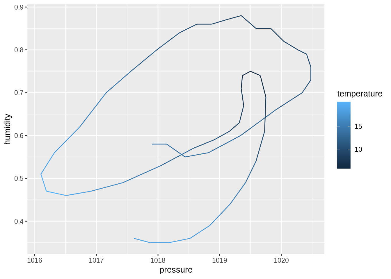
##
## $toronto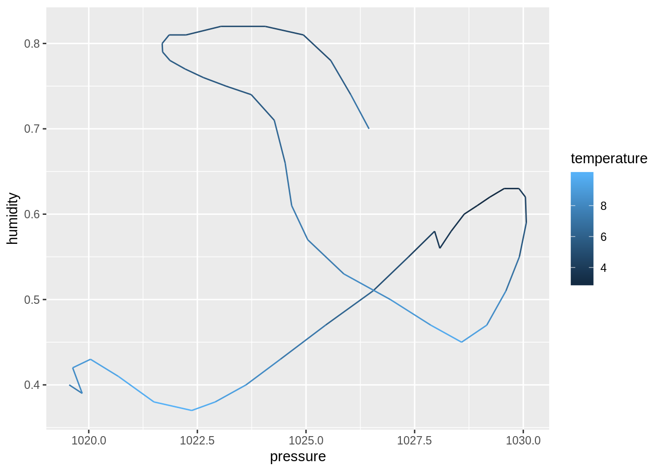
##
## $tel_aviv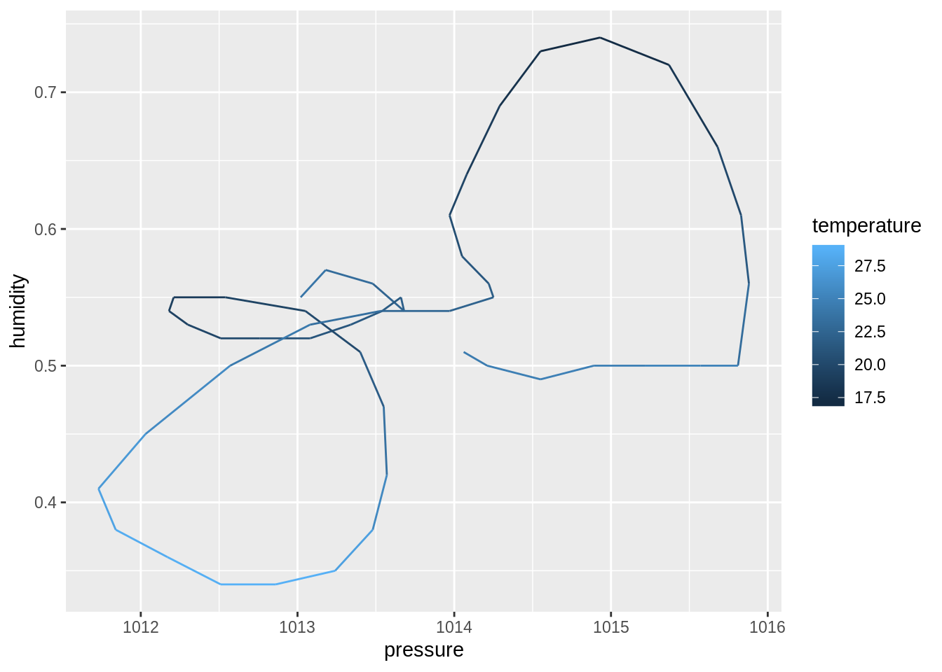
##
## $zurich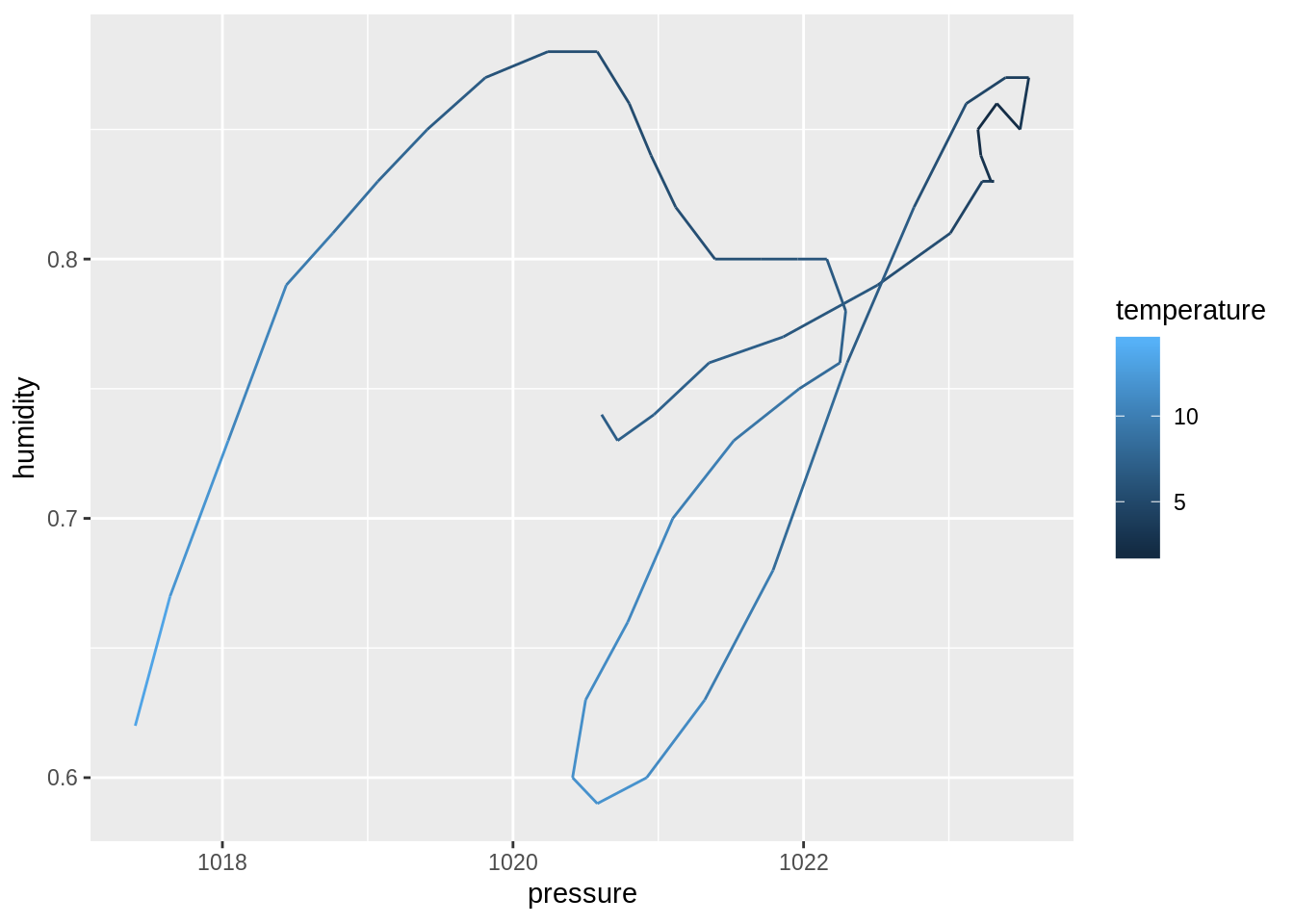
3.7 Typed output
Click here to show setup code.
library(tidyverse)
library(here)

dict <- readxl::read_excel(here("data/cities.xlsx"))

input_data <-
  dict %>%
  select(city_code, weather_filename) %>%
  deframe() %>%
  map(~ readxl::read_excel(here(.)))
If we know, what the output of each function call in a map() sequence looks like, we can often call a sub-type of map() to produce a more condensed output.
We start with the named list of tibbles called input_data from section “Processing all files”.
We want to know the number of rows of each tibble in input_data:
input_data %>%
  map(~ nrow(.))
## $berlin
## [1] 49
##
## $toronto
## [1] 49
##
## $tel_aviv
## [1] 49
##
## $zurich
## [1] 49Each time an integer is produced.
Therefore we can call map_int(), to create a named integer vector:
input_data %>%
  map_int(~ nrow(.))
## berlin toronto tel_aviv zurich
## 49 49 49 49If the output is of type character, use map_chr():
input_data %>%
  map_chr(~ nrow(.))
## berlin toronto tel_aviv zurich
## "49" "49" "49" "49"input_data %>%
map_chr(~ as.character(nrow(.)))## berlin toronto tel_aviv zurich
## "49" "49" "49" "49"There are sub-types of the map() function for each atomic type:
integer:
map_int()numeric (double-precision value):
map_dbl()character (strings):
map_chr()logical (flags):
map_lgl()raw (bytes):
map_raw()
3.7.1 Exercises
Explain what happens if you try to use
map_dbl()with thedim()output:input_data %>% map_dbl(dim)Extract a concise version of the first temperature value for each dataset:
input_data %>%
  map(~ slice(., 1)) %>%
  ___(~ pull(_____))
## berlin toronto tel_aviv zurich ## 13.43 7.46 23.90 6.96Use
paste0()to build a textual description for the weather during the observed period in a function. Create a two-column tibble.summarize_weather <- _____ { ___ %>% ___( _____, _____, _____, summary = paste(rle(summary)$values, collapse = ", then ") ) } describe_weather <- function(weather_summary) { weather_summary %>% mutate( text = paste0( "We had temperatures between ", min_temp, " and ", max_temp, " °C.", "The average humidity was ", round(mean_humidity * 100), " %. ", "The weather was ", summary, "." ) ) %>% pull() } input_data %>% ___(___) %>% ___(___) %>% ___()## # A tibble: 4 x 2 ## name value ## <chr> <chr> ## 1 berlin We had temperatures between 6.14 and 19.98 °C.The average humid… ## 2 toronto We had temperatures between 3.03 and 9.99 °C.The average humidi… ## 3 tel_aviv We had temperatures between 17.15 and 28.77 °C.The average humi… ## 4 zurich We had temperatures between 2.01 and 14.3 °C.The average humidi…
function
here::here()is taking care of making sure we start from the root directory of our current project↩