5 Tidying

Rows, columns, cells.

This chapter discusses pivoting and data tidying with the help of the tidyr package.

5.1 Pivoting

Click here to show setup code.

library(tidyverse)
library(nycflights13)

library(conflicted)
conflict_prefer("filter", "dplyr")

## [conflicted] Removing existing preference

## [conflicted] Will prefer [34mdplyr::filter[39m over any other package

conflict_prefer("lag", "dplyr")

## [conflicted] Removing existing preference

## [conflicted] Will prefer [34mdplyr::lag[39m over any other package

Pivoting describes operations that help rearrange data in different ways. The following two tables contain the same data arranged differently.

table1

## # A tibble: 6 x 4
##   country      year  cases population
##   <chr>       <int>  <int>      <int>
## 1 Afghanistan  1999    745   19987071
## 2 Afghanistan  2000   2666   20595360
## 3 Brazil       1999  37737  172006362
## 4 Brazil       2000  80488  174504898
## 5 China        1999 212258 1272915272
## 6 China        2000 213766 1280428583

table2

## # A tibble: 12 x 4
##   country      year type          count
##   <chr>       <int> <chr>         <int>
## 1 Afghanistan  1999 cases           745
## 2 Afghanistan  1999 population 19987071
## 3 Afghanistan  2000 cases          2666
## # … with 9 more rows

Both tables contain country and year column that describe the source of the measurements. The “wider” version, table1, contains two columns that hold the number of cases (of a disease) and the population for the corresponding country in the corresponding year. In the “longer” version, table2, the number of cases and the population are stored in the same count column, with the type column defining the measurement.

Somewhat counter-intuitively, “longer-form” data is often better suited for analyzing data. “Wider-form” data makes better use of screen space, but may be more difficult to work with.

The following example computes the maximum number of cases and population for each country. For the wider form, this requires repeating the same expression for all columns. This may work with two columns but becomes tedious once more measurements are added.

table1 %>%
  group_by(country) %>%
  summarize(
    max_cases = max(cases),
    max_population = max(population)
  ) %>%
  ungroup()

## # A tibble: 3 x 3
##   country     max_cases max_population
##   <chr>           <int>          <int>
## 1 Afghanistan      2666       20595360
## 2 Brazil          80488      174504898
## 3 China          213766     1280428583

The _at family of functions helps iterating over columns, but all columns still need to be enumerated. (Specifying ranges of columns is rather brittle.)

table1 %>%
  group_by(country) %>%
  summarize_at(
    vars(cases, population),
    max
  ) %>%
  ungroup()

## # A tibble: 3 x 3
##   country      cases population
##   <chr>        <int>      <int>
## 1 Afghanistan   2666   20595360
## 2 Brazil       80488  174504898
## 3 China       213766 1280428583

If the data is in the “longer” form, it is sufficient to include type in the grouping variables. The same code works for arbitrary number of measurements.

table2 %>%
  group_by(country, type) %>%
  summarize(
    max = max(count)
  ) %>%
  ungroup()

## # A tibble: 6 x 3
##   country     type              max
##   <chr>       <chr>           <int>
## 1 Afghanistan cases            2666
## 2 Afghanistan population   20595360
## 3 Brazil      cases           80488
## 4 Brazil      population  174504898
## 5 China       cases          213766
## 6 China       population 1280428583

The following examples give a gentle introduction into pivoting.

5.1.1 Convert to longer form

The pivot_longer() function takes a “wider-form” dataset and converts it to an equivalent dataset with more rows.

table1

## # A tibble: 6 x 4
##   country      year  cases population
##   <chr>       <int>  <int>      <int>
## 1 Afghanistan  1999    745   19987071
## 2 Afghanistan  2000   2666   20595360
## 3 Brazil       1999  37737  172006362
## 4 Brazil       2000  80488  174504898
## 5 China        1999 212258 1272915272
## 6 China        2000 213766 1280428583

table1 %>%
  pivot_longer(-c(country, year))

## # A tibble: 12 x 4
##   country      year name          value
##   <chr>       <int> <chr>         <int>
## 1 Afghanistan  1999 cases           745
## 2 Afghanistan  1999 population 19987071
## 3 Afghanistan  2000 cases          2666
## # … with 9 more rows

The -c(...) notation indicates that all column except country and year are to be transformed into longer form. The column names become the contents of the new name column, the values are available in the value column.

Your turn: The result of this operation isn’t strictly equivalent to table2. What is missing?

Alternatively, the names_to and values_to arguments allow specifying the names of the new columns.

try(
  table1 %>%
    pivot_longer(-c(country, year)) %>%
    select(....., everything())
)

## Error in .f(.x[[i]], ...) : object '.....' not found

table1 %>%
  pivot_longer(
    -c(country, year),
    names_to = "type",
    values_to = "count"
  )

## # A tibble: 12 x 4
##   country      year type          count
##   <chr>       <int> <chr>         <int>
## 1 Afghanistan  1999 cases           745
## 2 Afghanistan  1999 population 19987071
## 3 Afghanistan  2000 cases          2666
## # … with 9 more rows

5.1.2 Convert to wider form

The pivot_wider() form does the inverse: it creates a dataset with fewer rows. If the name and value columns are named differently, these columns can be provided via the names_from and values_from arguments.

table2

## # A tibble: 12 x 4
##   country      year type          count
##   <chr>       <int> <chr>         <int>
## 1 Afghanistan  1999 cases           745
## 2 Afghanistan  1999 population 19987071
## 3 Afghanistan  2000 cases          2666
## # … with 9 more rows

table2 %>%
  pivot_wider(names_from = type, values_from = count)

## # A tibble: 6 x 4
##   country      year  cases population
##   <chr>       <int>  <int>      <int>
## 1 Afghanistan  1999    745   19987071
## 2 Afghanistan  2000   2666   20595360
## 3 Brazil       1999  37737  172006362
## 4 Brazil       2000  80488  174504898
## 5 China        1999 212258 1272915272
## 6 China        2000 213766 1280428583

Your turn: pivot_wider() expects columns name and value by default. What do we need to do to get rid of names_from and values_from?

try(
  table2 %>%
    select(......, everything()) %>%
    pivot_wider()
)

## Error in .f(.x[[i]], ...) : object '......' not found

5.1.3 Use cases

Data in “longer” form usually works better for plotting the values side by side, e.g. by assigning the type of value to an aesthetic. Recall that each row in the data produces one geometric object in the corresponding layer. For a bar chart that shows cases and population side by side, mapped to the y aesthetic, the “longer” form is more natural.

table2 form requires only one layer, the fill color is determined automatically, the legend is created automatically
table1 requires two layers, manual assignment of fill color, and manual creation of legend (not shown)

table2 %>%
  ggplot() +
  geom_col(aes(country, count, fill = type), position = "dodge") +
  facet_wrap(~year) +
  scale_y_log10()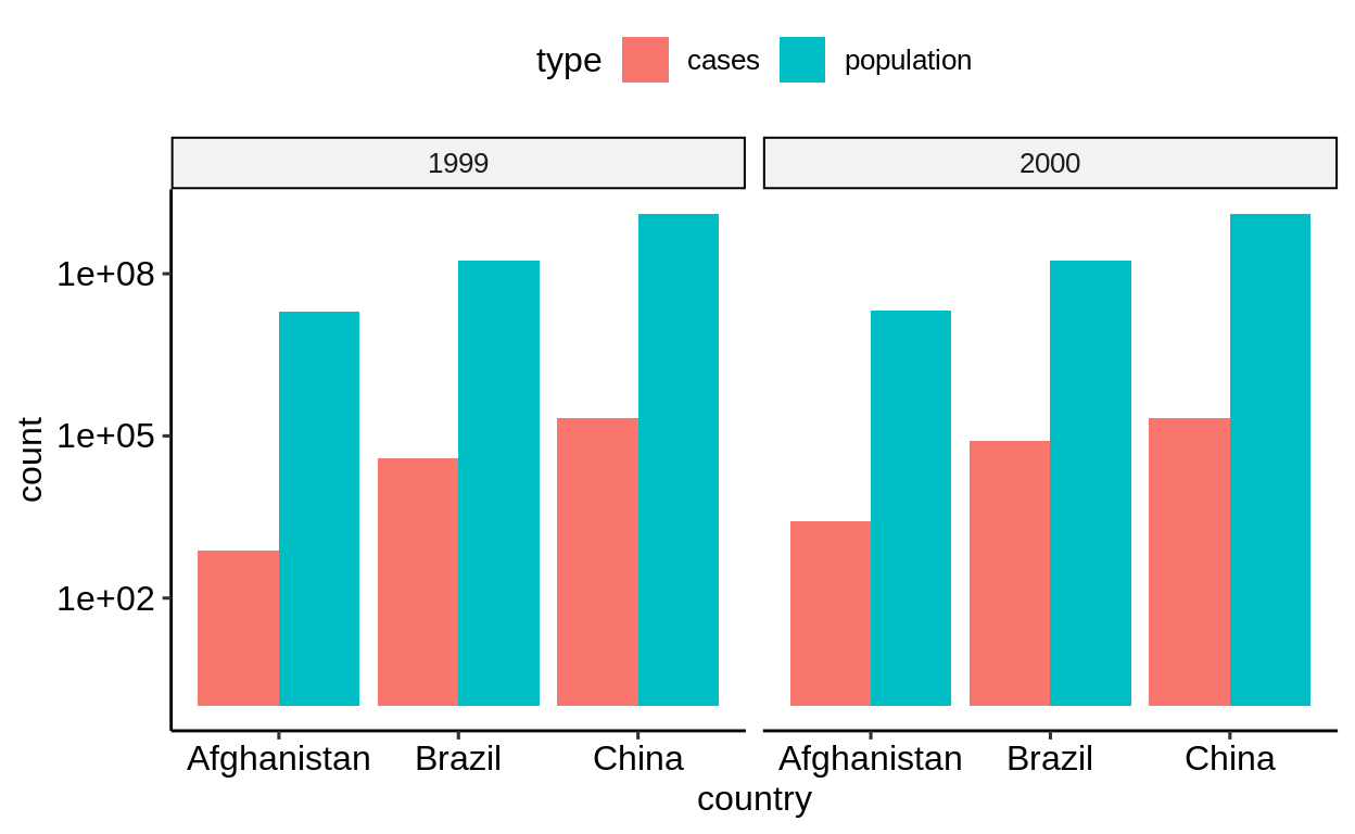

table1 %>%
  ggplot() +
  geom_col(aes(country, population), position = "dodge", fill = "blue") +
  geom_col(aes(country, cases), position = "dodge", fill = "red") +
  facet_wrap(~year) +
  scale_y_log10()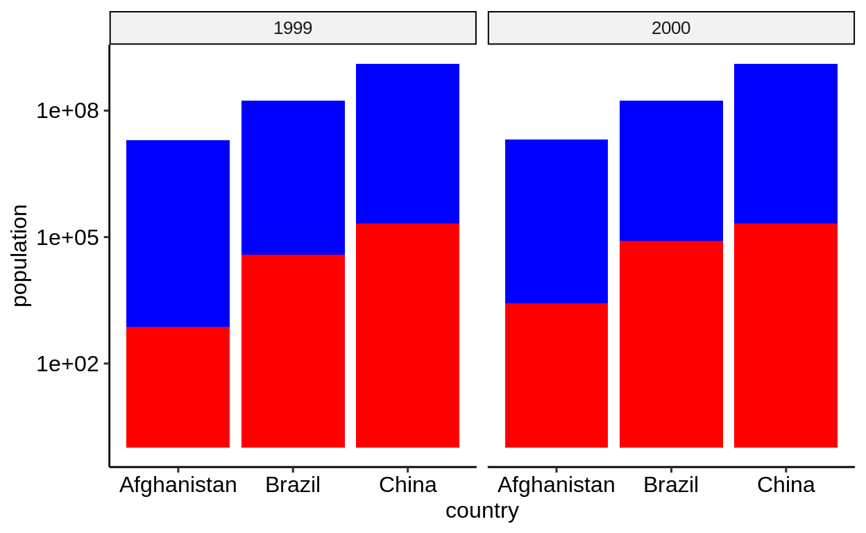

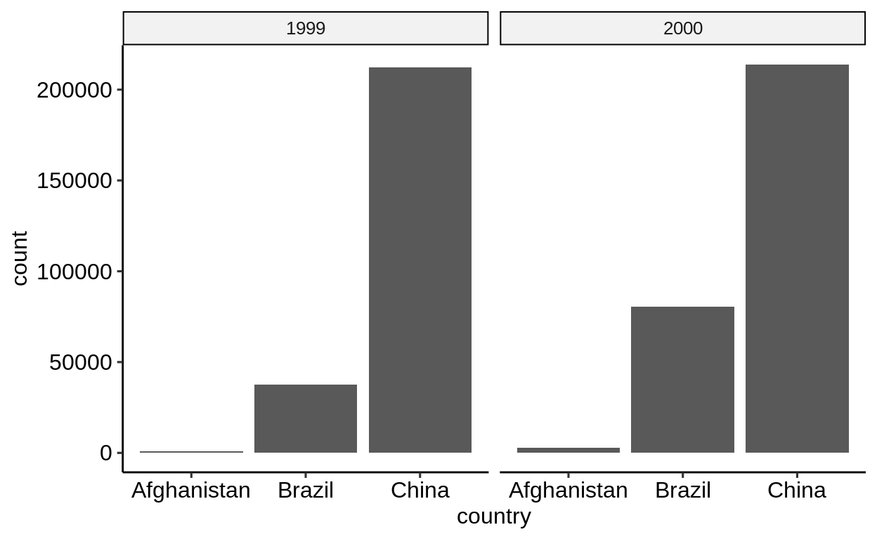
On the other hand, iIf only a single measurement needs to be plotted, the “wider” form is easier to work with.

table1 only requires selecting the correct column
table2 requires a filter()

table1 %>%
  ggplot() +
  geom_col(aes(country, cases)) +
  facet_wrap(~year)

table2 %>%
  filter(type == "cases") %>%
  ggplot() +
  geom_col(aes(country, count)) +
  facet_wrap(~year)

The “wider” form is also the only way to map different measures to different aesthetics, e.g. to correlate values.

table1 %>%
  ggplot() +
  geom_point(aes(cases, population, color = factor(year), shape = country)) +
  scale_x_log10() +
  scale_y_log10()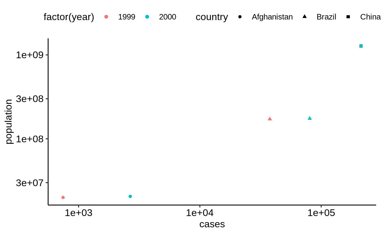

5.1.4 Combining vertically

A different view on the same data is given in the two tables table4a and table4b.

table4a

## # A tibble: 3 x 3
##   country     `1999` `2000`
## * <chr>        <int>  <int>
## 1 Afghanistan    745   2666
## 2 Brazil       37737  80488
## 3 China       212258 213766

table4b

## # A tibble: 3 x 3
##   country         `1999`     `2000`
## * <chr>            <int>      <int>
## 1 Afghanistan   19987071   20595360
## 2 Brazil       172006362  174504898
## 3 China       1272915272 1280428583

The bind_rows() function combines these two parts into a single table. The .id = "type" setting ensures that the input datasets gain different tags in the new type column.

table4 <-
  bind_rows(
    cases = table4a,
    population = table4b,
    .id = "type"
  )
table4

## # A tibble: 6 x 4
##   type       country         `1999`     `2000`
##   <chr>      <chr>            <int>      <int>
## 1 cases      Afghanistan        745       2666
## 2 cases      Brazil           37737      80488
## 3 cases      China           212258     213766
## 4 population Afghanistan   19987071   20595360
## 5 population Brazil       172006362  174504898
## 6 population China       1272915272 1280428583

Your turn: As before, pivot_longer() helps converting the results into something similar to table2. The result isn’t quite the same yet, can you spot the difference?

try(
  table4 %>%
    ...(c(.....))
)

## Error in ...(., c(.....)) : could not find function "..."

5.1.5 Tidy data

From “R for data science”:

In a tidy dataset,

each variable must have its own column.

each observation must have its own row.

each value must have its own cell.

Tidy data

The next two sections show examples of datasets that violate these principles.

5.1.6 The Anscombe dataset

This is a dataset where principal statistical summaries (means, standard deviations, intercept and slope after regression) are identical across four subgroups but the layout of the data differs vastly.

anscombe

##   x1 x2 x3 x4   y1   y2   y3   y4
## 1 10 10 10  8 8.04 9.14 7.46 6.58
## 2  8  8  8  8 6.95 8.14 6.77 5.76
##  [ reached 'max' / getOption("max.print") -- omitted 9 rows ]

anscombe %>%
  as_tibble()

## # A tibble: 11 x 8
##      x1    x2    x3    x4    y1    y2    y3    y4
##   <dbl> <dbl> <dbl> <dbl> <dbl> <dbl> <dbl> <dbl>
## 1    10    10    10     8  8.04  9.14  7.46  6.58
## 2     8     8     8     8  6.95  8.14  6.77  5.76
## 3    13    13    13     8  7.58  8.74 12.7   7.71
## # … with 8 more rows

Working with this data in original form is rather tedious.

anscombe %>%
  as_tibble() %>%
  summarize_all(list(~ mean(.), ~ sd(.)))

## # A tibble: 1 x 16
##   x1_mean x2_mean x3_mean x4_mean y1_mean y2_mean y3_mean
##     <dbl>   <dbl>   <dbl>   <dbl>   <dbl>   <dbl>   <dbl>
## 1       9       9       9       9    7.50    7.50     7.5
## # … with 9 more variables: y4_mean <dbl>, x1_sd <dbl>,
## #   x2_sd <dbl>, x3_sd <dbl>, x4_sd <dbl>, y1_sd <dbl>,
## #   y2_sd <dbl>, y3_sd <dbl>, y4_sd <dbl>

lm(y1 ~ x1, anscombe)

## 
## Call:
## lm(formula = y1 ~ x1, data = anscombe)
## 
## Coefficients:
## (Intercept)           x1  
##      3.0001       0.5001

lm(y2 ~ x2, anscombe)

## 
## Call:
## lm(formula = y2 ~ x2, data = anscombe)
## 
## Coefficients:
## (Intercept)           x2  
##       3.001        0.500

lm(y3 ~ x3, anscombe)

## 
## Call:
## lm(formula = y3 ~ x3, data = anscombe)
## 
## Coefficients:
## (Intercept)           x3  
##      3.0025       0.4997

lm(y4 ~ x4, anscombe)

## 
## Call:
## lm(formula = y4 ~ x4, data = anscombe)
## 
## Coefficients:
## (Intercept)           x4  
##      3.0017       0.4999

try(
  ggplot(anscombe) + 
    ...
)

## Error in try(ggplot(anscombe) + ...) : '...' used in an incorrect context

Your turn: Which principles of tidy data does the anscombe dataset violate?

Many operations become much more natural when the data is in longer form.

anscombe_longer <-
  anscombe %>%
  mutate(id = row_number()) %>%
  pivot_longer(
    -id,
    names_pattern = "(.)(.)",
    names_to = c(".value", "measurement")
  ) %>%
  arrange(measurement, id)

anscombe_longer %>%
  group_by(measurement) %>%
  summarize_at(vars(x, y), list(~ mean(.), ~sd(.))) %>%
  ungroup()

## # A tibble: 4 x 5
##   measurement x_mean y_mean  x_sd  y_sd
##   <chr>        <dbl>  <dbl> <dbl> <dbl>
## 1 1                9   7.50  3.32  2.03
## 2 2                9   7.50  3.32  2.03
## 3 3                9   7.5   3.32  2.03
## 4 4                9   7.50  3.32  2.03

anscombe_longer %>%
  group_by(measurement) %>%
  summarize(model = list(lm(y ~ x, .))) %>%
  ungroup() %>%
  pull()

## [[1]]
## 
## Call:
## lm(formula = y ~ x, data = .)
## 
## Coefficients:
## (Intercept)            x  
##      3.0013       0.4999  
## 
## 
## [[2]]
## 
## Call:
## lm(formula = y ~ x, data = .)
## 
## Coefficients:
## (Intercept)            x  
##      3.0013       0.4999  
## 
## 
## [[3]]
## 
## Call:
## lm(formula = y ~ x, data = .)
## 
## Coefficients:
## (Intercept)            x  
##      3.0013       0.4999  
## 
## 
## [[4]]
## 
## Call:
## lm(formula = y ~ x, data = .)
## 
## Coefficients:
## (Intercept)            x  
##      3.0013       0.4999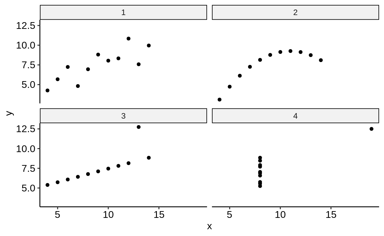

anscombe_longer %>%
  ggplot(aes(x = x, y = y)) +
  geom_point() +
  facet_wrap(vars(measurement))

5.1.7 WHO data

The following example shows a case that violates the first two rules of tidy data: WHO data arranged for optimal use of screen space. The column names define, in addition to the measurement type new_sp, new_sn, new_ep and newrel, the age and sex stratum of the corresponding measurements. One single pivot_longer() call transforms the data into a longer-form version with four measurement columns and one row for each age/sex stratum. The names_pattern is a regular expression that defines what part of the column name is stored where. (Regular expressions are a powerful tool for parsing text data, out of scope for this lecture but very much worth looking into.) The names_to sequence defines, for each () group in names_pattern, if the data encoded in the column name is stored in a new column or if it is kept as column name.

who %>%
  view()

## # A tibble: 7,240 x 60
##   country iso2  iso3   year new_sp_m014 new_sp_m1524
##   <chr>   <chr> <chr> <int>       <int>        <int>
## 1 Afghan… AF    AFG    1980          NA           NA
## 2 Afghan… AF    AFG    1981          NA           NA
## 3 Afghan… AF    AFG    1982          NA           NA
## # … with 7,237 more rows, and 54 more variables:
## #   new_sp_m2534 <int>, new_sp_m3544 <int>,
## #   new_sp_m4554 <int>, new_sp_m5564 <int>, new_sp_m65 <int>,
## #   new_sp_f014 <int>, new_sp_f1524 <int>,
## #   new_sp_f2534 <int>, new_sp_f3544 <int>,
## #   new_sp_f4554 <int>, new_sp_f5564 <int>, new_sp_f65 <int>,
## #   new_sn_m014 <int>, new_sn_m1524 <int>,
## #   new_sn_m2534 <int>, new_sn_m3544 <int>,
## #   new_sn_m4554 <int>, new_sn_m5564 <int>, new_sn_m65 <int>,
## #   new_sn_f014 <int>, new_sn_f1524 <int>,
## #   new_sn_f2534 <int>, new_sn_f3544 <int>,
## #   new_sn_f4554 <int>, new_sn_f5564 <int>, new_sn_f65 <int>,
## #   new_ep_m014 <int>, new_ep_m1524 <int>,
## #   new_ep_m2534 <int>, new_ep_m3544 <int>,
## #   new_ep_m4554 <int>, new_ep_m5564 <int>, new_ep_m65 <int>,
## #   new_ep_f014 <int>, new_ep_f1524 <int>,
## #   new_ep_f2534 <int>, new_ep_f3544 <int>,
## #   new_ep_f4554 <int>, new_ep_f5564 <int>, new_ep_f65 <int>,
## #   newrel_m014 <int>, newrel_m1524 <int>,
## #   newrel_m2534 <int>, newrel_m3544 <int>,
## #   newrel_m4554 <int>, newrel_m5564 <int>, newrel_m65 <int>,
## #   newrel_f014 <int>, newrel_f1524 <int>,
## #   newrel_f2534 <int>, newrel_f3544 <int>,
## #   newrel_f4554 <int>, newrel_f5564 <int>, newrel_f65 <int>

who_longer <-
  who %>%
  pivot_longer(
    -(country:year),
    names_pattern = "([a-z_]+)_(.)([0-9]+)",
    names_to = c(".value", "sex", "age")
  )

who_longer

## # A tibble: 101,360 x 10
##   country iso2  iso3   year sex   age   new_sp new_sn new_ep
##   <chr>   <chr> <chr> <int> <chr> <chr>  <int>  <int>  <int>
## 1 Afghan… AF    AFG    1980 m     014       NA     NA     NA
## 2 Afghan… AF    AFG    1980 m     1524      NA     NA     NA
## 3 Afghan… AF    AFG    1980 m     2534      NA     NA     NA
## # … with 1.014e+05 more rows, and 1 more variable:
## #   newrel <int>

who_longer %>%
  count(sex, age)

## # A tibble: 14 x 3
##   sex   age       n
##   <chr> <chr> <int>
## 1 f     014    7240
## 2 f     1524   7240
## 3 f     2534   7240
## # … with 11 more rows

5.1.8 Formatting tables for presentation

Wide tables make better use of screen or paper space, and should be used when presenting tables that summarize across multiple dimensions. For this, ftable() is the better tool.

table2 %>%
  xtabs(count ~ ., .) %>%
  ftable()

##                  type      cases population
## country     year                           
## Afghanistan 1999             745   19987071
##             2000            2666   20595360
## Brazil      1999           37737  172006362
##             2000           80488  174504898
## China       1999          212258 1272915272
##             2000          213766 1280428583

These can be converted to HTML for inclusion in reports, e.g. with memisc::format_html().

table2_html <-
  table2 %>%
  xtabs(count ~ ., .) %>%
  ftable(col.vars = c("year", "type")) %>% 
  memisc::format_html()

cat(table2_html)

	year:	1999		2000
country	type:	cases	population	cases	population
Afghanistan		745	19987071	2666	20595360
Brazil		37737	172006362	80488	174504898
China		212258	1272915272	213766	1280428583

The {gt} package is a modern approach to present tables for formatting.

5.2 Separating and uniting

Click here to show setup code.

library(tidyverse)
library(nycflights13)

library(conflicted)
conflict_prefer("filter", "dplyr")

## [conflicted] Removing existing preference

## [conflicted] Will prefer [34mdplyr::filter[39m over any other package

conflict_prefer("lag", "dplyr")

## [conflicted] Removing existing preference

## [conflicted] Will prefer [34mdplyr::lag[39m over any other package

The table3 table violates the third principle of tidy data: each cell in the rate column contains two values.

table3

## # A tibble: 6 x 3
##   country      year rate             
## * <chr>       <int> <chr>            
## 1 Afghanistan  1999 745/19987071     
## 2 Afghanistan  2000 2666/20595360    
## 3 Brazil       1999 37737/172006362  
## 4 Brazil       2000 80488/174504898  
## 5 China        1999 212258/1272915272
## 6 China        2000 213766/1280428583

The separate() verb offers a convenient way to deal with this situation, including automatic type conversion.

table3 %>%
  separate(rate, into = c("cases", "population"))

## # A tibble: 6 x 4
##   country      year cases  population
##   <chr>       <int> <chr>  <chr>     
## 1 Afghanistan  1999 745    19987071  
## 2 Afghanistan  2000 2666   20595360  
## 3 Brazil       1999 37737  172006362 
## 4 Brazil       2000 80488  174504898 
## 5 China        1999 212258 1272915272
## 6 China        2000 213766 1280428583

table3 %>%
  separate(rate, into = c("cases", "population"), sep = "/", convert = TRUE)

## # A tibble: 6 x 4
##   country      year  cases population
##   <chr>       <int>  <int>      <int>
## 1 Afghanistan  1999    745   19987071
## 2 Afghanistan  2000   2666   20595360
## 3 Brazil       1999  37737  172006362
## 4 Brazil       2000  80488  174504898
## 5 China        1999 212258 1272915272
## 6 China        2000 213766 1280428583

The inverse is offered by unite(). The data in table5 stores year data in two columns.

table5

## # A tibble: 6 x 4
##   country     century year  rate             
## * <chr>       <chr>   <chr> <chr>            
## 1 Afghanistan 19      99    745/19987071     
## 2 Afghanistan 20      00    2666/20595360    
## 3 Brazil      19      99    37737/172006362  
## 4 Brazil      20      00    80488/174504898  
## 5 China       19      99    212258/1272915272
## 6 China       20      00    213766/1280428583

table5 %>%
  unite("year", c(century, year))

## # A tibble: 6 x 3
##   country     year  rate             
##   <chr>       <chr> <chr>            
## 1 Afghanistan 19_99 745/19987071     
## 2 Afghanistan 20_00 2666/20595360    
## 3 Brazil      19_99 37737/172006362  
## 4 Brazil      20_00 80488/174504898  
## 5 China       19_99 212258/1272915272
## 6 China       20_00 213766/1280428583

The result needs a few tweaks to finally resemble table3.

table5 %>%
  unite("year", c(century, year), sep = "")

## # A tibble: 6 x 3
##   country     year  rate             
##   <chr>       <chr> <chr>            
## 1 Afghanistan 1999  745/19987071     
## 2 Afghanistan 2000  2666/20595360    
## 3 Brazil      1999  37737/172006362  
## 4 Brazil      2000  80488/174504898  
## 5 China       1999  212258/1272915272
## 6 China       2000  213766/1280428583

table5 %>%
  unite("year", c(century, year), sep = "") %>%
  mutate(year = as.numeric(year))

## # A tibble: 6 x 3
##   country      year rate             
##   <chr>       <dbl> <chr>            
## 1 Afghanistan  1999 745/19987071     
## 2 Afghanistan  2000 2666/20595360    
## 3 Brazil       1999 37737/172006362  
## 4 Brazil       2000 80488/174504898  
## 5 China        1999 212258/1272915272
## 6 China        2000 213766/1280428583

See the help for further details.

?separate
?unite

5.2.1 Parsing numbers

thousand_separator <-
  tribble(
    ~num,
    "1'000.00",
    "2'000'000.00"
  )

thousand_separator

## # A tibble: 2 x 1
##   num         
##   <chr>       
## 1 1'000.00    
## 2 2'000'000.00

thousand_separator %>%
  separate(num, into = c("num"))

## Warning: Expected 1 pieces. Additional pieces discarded in 2
## rows [1, 2].

## # A tibble: 2 x 1
##   num  
##   <chr>
## 1 1    
## 2 2

thousand_separator %>%
  mutate(num = str_replace_all(num, "[^-0-9.]", "")) %>%
  mutate(num = as.numeric(num))

## # A tibble: 2 x 1
##       num
##     <dbl>
## 1    1000
## 2 2000000