Spreading and gathering
Kirill Müller, cynkra GmbH
June 2, 2017
table2 to table1
table2 %>%
  spread(type, count)
## # A tibble: 6 x 4
## country year cases population
## <chr> <int> <int> <int>
## 1 Afghanistan 1999 745 19987071
## 2 Afghanistan 2000 2666 20595360
## 3 Brazil 1999 37737 172006362
## 4 Brazil 2000 80488 174504898
## 5 China 1999 212258 1272915272
## 6 China 2000 213766 1280428583table1 to table2
table1 %>%
  gather(type, count, cases, population)
## # A tibble: 12 x 4
## country year type count
## <chr> <int> <chr> <int>
## 1 Afghanistan 1999 cases 745
## 2 Afghanistan 2000 cases 2666
## 3 Brazil 1999 cases 37737
## 4 Brazil 2000 cases 80488
## 5 China 1999 cases 212258
## 6 China 2000 cases 213766
## 7 Afghanistan 1999 population 19987071
## 8 Afghanistan 2000 population 20595360
## 9 Brazil 1999 population 172006362
## 10 Brazil 2000 population 174504898
## 11 China 1999 population 1272915272
## 12 China 2000 population 1280428583table2 %>%
gather(type, count, -country, -year)## # A tibble: 24 x 4
## country year type count
## <chr> <int> <chr> <chr>
## 1 Afghanistan 1999 type cases
## 2 Afghanistan 1999 type population
## 3 Afghanistan 2000 type cases
## 4 Afghanistan 2000 type population
## 5 Brazil 1999 type cases
## 6 Brazil 1999 type population
## 7 Brazil 2000 type cases
## 8 Brazil 2000 type population
## 9 China 1999 type cases
## 10 China 1999 type population
## # ... with 14 more rowsAre the two calls symmetrical?
No, we need to arrange this result:
table1 %>%
  gather(type, count, -country, -year) %>%
  arrange(country, year, type)
## # A tibble: 12 x 4
## country year type count
## <chr> <int> <chr> <int>
## 1 Afghanistan 1999 cases 745
## 2 Afghanistan 1999 population 19987071
## 3 Afghanistan 2000 cases 2666
## 4 Afghanistan 2000 population 20595360
## 5 Brazil 1999 cases 37737
## 6 Brazil 1999 population 172006362
## 7 Brazil 2000 cases 80488
## 8 Brazil 2000 population 174504898
## 9 China 1999 cases 212258
## 10 China 1999 population 1272915272
## 11 China 2000 cases 213766
## 12 China 2000 population 1280428583Plot table-x
For showing one measurement:
table1 %>%
  ggplot(aes(country, population, fill = factor(year))) +
  geom_col(position = "dodge")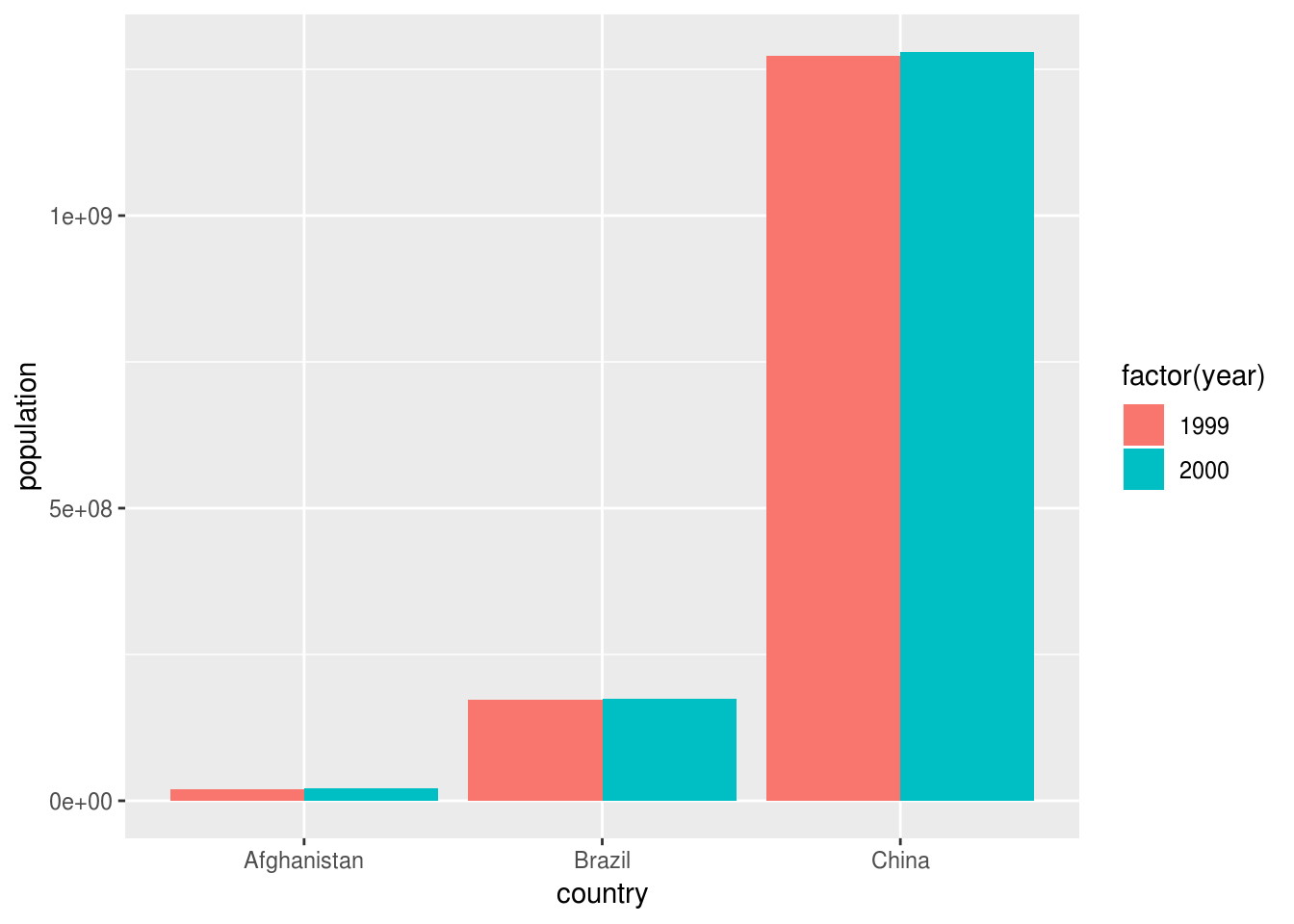
For mapping measurement type to an aesthetic:
table2 %>%
  ggplot(aes(country, count, fill = type)) +
  geom_col() +
  facet_wrap(~year)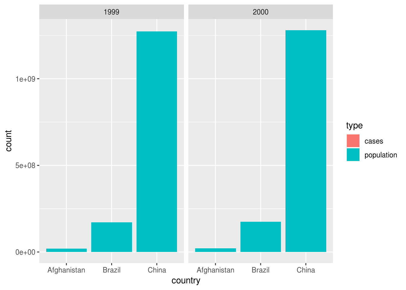
For mapping both measurements to two aesthetics:
table1 %>%
  ggplot(aes(population, cases, color = country)) +
  geom_point() +
  facet_wrap(~year)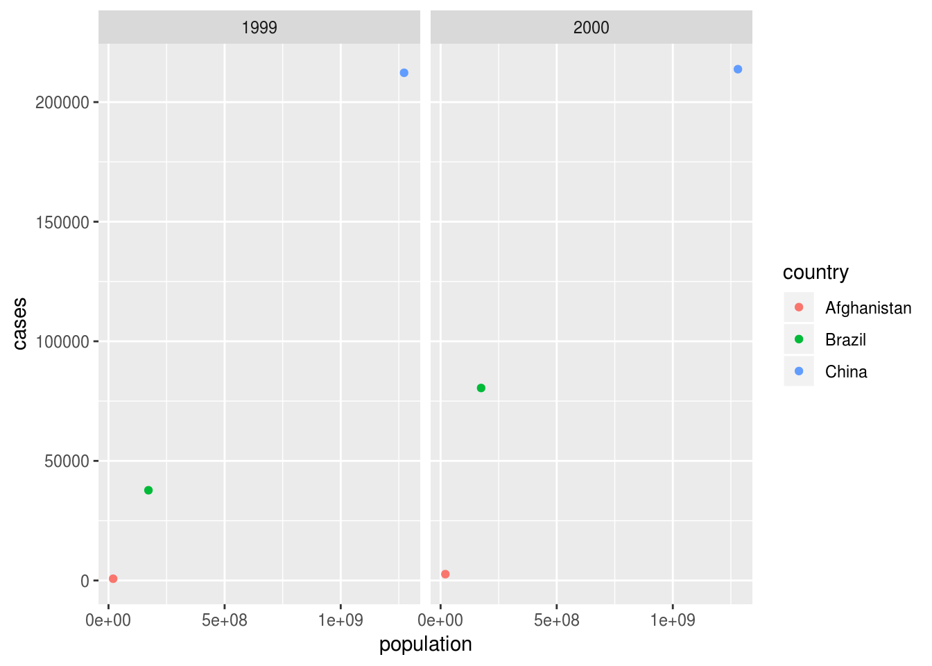
Can also use table1 to show only one measurement:
table2 %>%
  filter(type == "cases") %>%
  ggplot() +
  geom_col(aes(country, count, fill = type)) +
  facet_wrap(~year)
Binding
cases_tbl <-
  table4a %>%
  gather(year, count, -country) %>%
  mutate(type = "cases")

population_tbl <-
  table4b %>%
  gather(year, count, -country) %>%
  mutate(type = "population")

bind_rows(cases_tbl, population_tbl) %>%
  select(country, year, everything()) %>%
  arrange(country, year, type)
## # A tibble: 12 x 4
## country year count type
## <chr> <chr> <int> <chr>
## 1 Afghanistan 1999 745 cases
## 2 Afghanistan 1999 19987071 population
## 3 Afghanistan 2000 2666 cases
## 4 Afghanistan 2000 20595360 population
## 5 Brazil 1999 37737 cases
## 6 Brazil 1999 172006362 population
## 7 Brazil 2000 80488 cases
## 8 Brazil 2000 174504898 population
## 9 China 1999 212258 cases
## 10 China 1999 1272915272 population
## 11 China 2000 213766 cases
## 12 China 2000 1280428583 populationWith just one call to gather():
cases_tbl <-
  table4a %>%
  mutate(type = "cases")

population_tbl <-
  table4b %>%
  mutate(type = "population")

bind_rows(cases_tbl, population_tbl) %>%
  gather(year, count, -country, -type) %>%
  select(country, year, everything()) %>%
  arrange(country, year, type)
## # A tibble: 12 x 4
## country year type count
## <chr> <chr> <chr> <int>
## 1 Afghanistan 1999 cases 745
## 2 Afghanistan 1999 population 19987071
## 3 Afghanistan 2000 cases 2666
## 4 Afghanistan 2000 population 20595360
## 5 Brazil 1999 cases 37737
## 6 Brazil 1999 population 172006362
## 7 Brazil 2000 cases 80488
## 8 Brazil 2000 population 174504898
## 9 China 1999 cases 212258
## 10 China 1999 population 1272915272
## 11 China 2000 cases 213766
## 12 China 2000 population 1280428583Economies
mpg %>%
  select(displ, hwy, cty) %>%
  gather(cty_hwy, value, hwy, cty) %>%
  ggplot() +
  geom_jitter(aes(displ, value, color = cty_hwy))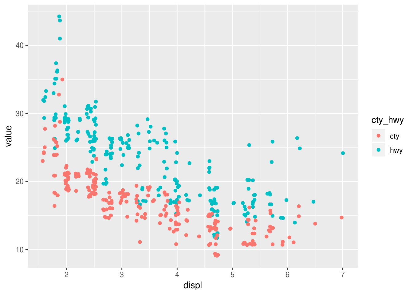
Copyright © 2018 Kirill Müller. Licensed under CC BY-NC 4.0.