Summarize
Kirill Müller, cynkra GmbH
Count flights
How many flights departed in New York City in 2013?
flights %>%
  count()
► Solution:
flights %>%
  count()
## # A tibble: 1 x 1
## n
## <int>
## 1 336776This is different to nrow():
flights %>%
  nrow()
## [1] 336776Count flights per airline
How many flights did each airline fly out of New York City in 2013?
flights %>%
  count(___)
► Solution:
flights %>%
  count(carrier)
## # A tibble: 16 x 2
## carrier n
## <chr> <int>
## 1 9E 18460
## 2 AA 32729
## 3 AS 714
## 4 B6 54635
## 5 DL 48110
## 6 EV 54173
## 7 F9 685
## 8 FL 3260
## 9 HA 342
## 10 MQ 26397
## 11 OO 32
## 12 UA 58665
## 13 US 20536
## 14 VX 5162
## 15 WN 12275
## 16 YV 601Sum up distance per airline
What’s the total distance flown for all flights originating in New York City in 2013, per airline?
flights %>%
  count(___, _____)
► Solution:
flights %>%
  count(carrier, wt = distance)
## # A tibble: 16 x 2
## carrier n
## <chr> <dbl>
## 1 9E 9788152
## 2 AA 43864584
## 3 AS 1715028
## 4 B6 58384137
## 5 DL 59507317
## 6 EV 30498951
## 7 F9 1109700
## 8 FL 2167344
## 9 HA 1704186
## 10 MQ 15033955
## 11 OO 16026
## 12 UA 89705524
## 13 US 11365778
## 14 VX 12902327
## 15 WN 12229203
## 16 YV 225395Useful summary functions
sum(),prod()mean(),median()sd(),IQR(),mad()min(),quantile(),max()n()sum()andmean()for logical variablesfirst(),last(),nth()
Don’t forget na.rm = TRUE if needed!
Mean arrival and dep delay
Compute the mean arrival and departure delay overall, and per origin airport. What is the standard deviation of these variables? What is New York City’s busiest airport?
flights %>%
  summarize(
    mean(___, na.rm = ___),
    _____,
    _____,
    _____
  )

flights %>%
  group_by(___) %>%
  summarize(_______)

flights %>%
  count(___) %>%
  arrange(___)
► Solution:
flights %>%
  summarize(
    mean(arr_delay, na.rm = TRUE),
    mean(dep_delay, na.rm = TRUE),
    sd(arr_delay, na.rm = TRUE),
    sd(dep_delay, na.rm = TRUE)
  )
## # A tibble: 1 x 4
## `mean(arr_delay, n… `mean(dep_delay, n… `sd(arr_delay, na.… `sd(dep_delay, na…
## <dbl> <dbl> <dbl> <dbl>
## 1 6.90 12.6 44.6 40.2flights %>%
summarize_at(
vars(arr_delay, dep_delay),
list(~ mean(., na.rm = TRUE), ~ sd(., na.rm = TRUE))
)## # A tibble: 1 x 4
## arr_delay_mean dep_delay_mean arr_delay_sd dep_delay_sd
## <dbl> <dbl> <dbl> <dbl>
## 1 6.90 12.6 44.6 40.2flights %>%
group_by(origin) %>%
summarize(
mean(arr_delay, na.rm = TRUE),
mean(dep_delay, na.rm = TRUE)
)## # A tibble: 3 x 3
## origin `mean(arr_delay, na.rm = TRUE)` `mean(dep_delay, na.rm = TRUE)`
## <chr> <dbl> <dbl>
## 1 EWR 9.11 15.1
## 2 JFK 5.55 12.1
## 3 LGA 5.78 10.3flights %>%
count(origin) %>%
arrange(desc(n))## # A tibble: 3 x 2
## origin n
## <chr> <int>
## 1 EWR 120835
## 2 JFK 111279
## 3 LGA 104662flights %>%
count(origin, sort = TRUE)## # A tibble: 3 x 2
## origin n
## <chr> <int>
## 1 EWR 120835
## 2 JFK 111279
## 3 LGA 104662Air time by carrier
Which carriers had the longest accumulated air time, excluding cancelled flights?
total_airtime_by_carrier <-
  flights %>%
  group_by(___) %>%
  summarize(acc_air_time = sum(_____)) %>%
  ungroup()

total_airtime_by_carrier
► Solution:
total_airtime_by_carrier <-
  flights %>%
  group_by(carrier) %>%
  summarize(acc_air_time = sum(air_time, na.rm = TRUE)) %>%
  ungroup()

total_airtime_by_carrier
## # A tibble: 16 x 2
## carrier acc_air_time
## <chr> <dbl>
## 1 9E 1500801
## 2 AA 6032306
## 3 AS 230863
## 4 B6 8170975
## 5 DL 8277661
## 6 EV 4603614
## 7 F9 156357
## 8 FL 321132
## 9 HA 213096
## 10 MQ 2282880
## 11 OO 2421
## 12 UA 12237728
## 13 US 1756507
## 14 VX 1724104
## 15 WN 1780402
## 16 YV 35763Air time by carrier, visualized
Plot a bar chart of the accumulated air time per airline, with a suitable unit for the total time.
Hint: Use fct_inorder() to fix the ordering of a categorical variable before plotting.
total_airtime_by_carrier <-
  _____

total_airtime_by_carrier %>%
  arrange(acc_air_time) %>%
  mutate(carrier = fct_inorder(carrier)) %>%
  ggplot(aes(___)) +
    geom_col()
► Solution:
total_airtime_by_carrier %>%
  arrange(acc_air_time) %>%
  mutate(carrier = fct_inorder(carrier)) %>%
  ggplot() +
  geom_col(aes(carrier, acc_air_time / 60 / 24 / 365)) +
  coord_flip()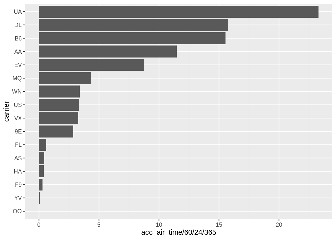
Carriers for long-distance routes
Which carriers specialize on long-distance routes?
mean_miles_by_carrier <-
  flights
  _____ %>%
  _____ %>%
  _____

mean_miles_by_carrier %>%
  arrange(_____)
► Solution:
mean_miles_by_carrier <-
  flights %>%
  group_by(carrier) %>%
  summarize(mean_distance = mean(distance)) %>%
  ungroup()

mean_miles_by_carrier %>%
  arrange(desc(mean_distance))
## # A tibble: 16 x 2
## carrier mean_distance
## <chr> <dbl>
## 1 HA 4983
## 2 VX 2499.
## 3 AS 2402
## 4 F9 1620
## 5 UA 1529.
## 6 AA 1340.
## 7 DL 1237.
## 8 B6 1069.
## 9 WN 996.
## 10 FL 665.
## 11 MQ 570.
## 12 EV 563.
## 13 US 553.
## 14 9E 530.
## 15 OO 501.
## 16 YV 375.Mean distance, visualized
Plot a bar chart of mean distance per flight. Use fct_inorder() to avoid sorting the axes. Do you use geom_bar() or geom_col()? Why?
mean_miles_by_carrier <-
  _____ %>%
  _____ %>%
  _____

mean_miles_by_carrier %>%
  arrange(_____) %>%
  mutate(___ = fct_inorder(___)) %>%
  ggplot(aes(_____)) +
    geom____()
► Solution:
We need geom_col(), because the data is already aggregated and contains one row per geometry object we’re plotting.
mean_miles_by_carrier <-
  flights %>%
  group_by(carrier) %>%
  summarize(mean_distance = mean(distance)) %>%
  ungroup()

mean_miles_by_carrier %>%
  arrange(desc(mean_distance)) %>%
  mutate(carrier = fct_inorder(carrier)) %>%
  ggplot() +
  geom_col(aes(x = carrier, y = mean_distance))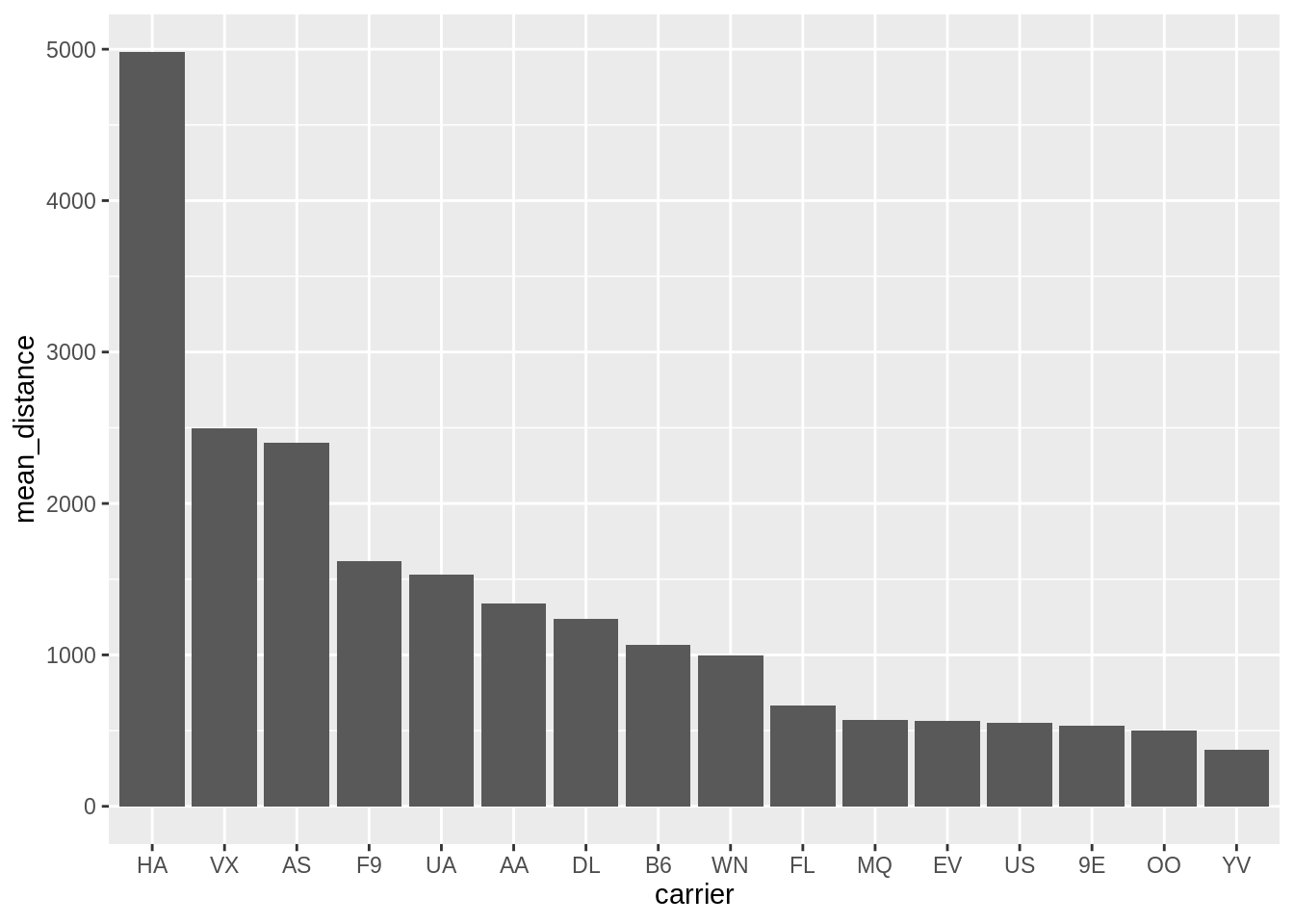
Worst plane
Which plane had the most failed departure attempts? Can you find a solution without filter()?
Hint: Use the idiom sum(___) to count the rows where a predicate is true.
flights %>%
  filter(is.na(dep_time)) %>%
  group_by(tailnum) %>%
  _____ %>%
  _____ %>%
  filter(!is.na(tailnum)) %>%
  arrange(desc(___)) %>%
  head(1)

# Alternative without filter():
flights %>%
  group_by(tailnum) %>%
  _____ %>%
  _____ %>%
  arrange(_____) %>%
  head(1)
► Solution:
flights %>%
  filter(is.na(dep_time)) %>%
  group_by(tailnum) %>%
  summarize(not_departed = n()) %>%
  ungroup() %>%
  filter(!is.na(tailnum)) %>%
  arrange(desc(not_departed))
## # A tibble: 1,449 x 2
## tailnum not_departed
## <chr> <int>
## 1 N725MQ 29
## 2 N713MQ 28
## 3 N723MQ 27
## 4 N15574 26
## 5 N722MQ 26
## 6 N13949 24
## 7 N14573 24
## 8 N735MQ 24
## 9 N11535 23
## 10 N11565 23
## # … with 1,439 more rowsShort-distance routes per airline, visualized
Compute the ratio of short-distance routes (less than 300 miles) for each airline.
Hint: Use the idiom mean(___) to compute the share of rows where a predicate is true.
flights %>%
  group_by(carrier) %>%
  _____ %>%
  ungroup()
► Solution:
flights %>%
  group_by(tailnum) %>%
  summarize(not_departed = sum(is.na(dep_time))) %>%
  ungroup()
## # A tibble: 4,044 x 2
## tailnum not_departed
## <chr> <int>
## 1 D942DN 0
## 2 N0EGMQ 17
## 3 N10156 7
## 4 N102UW 0
## 5 N103US 0
## 6 N104UW 0
## 7 N10575 17
## 8 N105UW 0
## 9 N107US 0
## 10 N108UW 0
## # … with 4,034 more rowsAn alternative, using filter() and count():
flights %>%
  filter(is.na(dep_time)) %>%
  count(tailnum, sort = TRUE)
## # A tibble: 1,450 x 2
## tailnum n
## <chr> <int>
## 1 <NA> 2512
## 2 N725MQ 29
## 3 N713MQ 28
## 4 N723MQ 27
## 5 N15574 26
## 6 N722MQ 26
## 7 N13949 24
## 8 N14573 24
## 9 N735MQ 24
## 10 N11535 23
## # … with 1,440 more rowsShort-distance routes per airline
Plot a bar chart of the ratio of short-distance routes.
short_distance_route_ratio <-
  _____

short_distance_route_ratio %>%
  ggplot(aes(___)) +
    geom_col()
► Solution:
short_distance_route_ratio <-
  flights %>%
  group_by(carrier) %>%
  summarize(short_distance_ratio = mean(distance < 300)) %>%
  ungroup() %>%
  arrange(desc(short_distance_ratio))

short_distance_route_ratio
## # A tibble: 16 x 2
## carrier short_distance_ratio
## <chr> <dbl>
## 1 YV 0.531
## 2 US 0.469
## 3 9E 0.313
## 4 EV 0.288
## 5 B6 0.198
## 6 MQ 0.111
## 7 UA 0.0572
## 8 AA 0.0445
## 9 OO 0.0312
## 10 DL 0.0252
## 11 WN 0.0169
## 12 AS 0
## 13 F9 0
## 14 FL 0
## 15 HA 0
## 16 VX 0short_distance_route_ratio %>%
ggplot() +
geom_col(aes(x = fct_inorder(carrier), y = short_distance_ratio))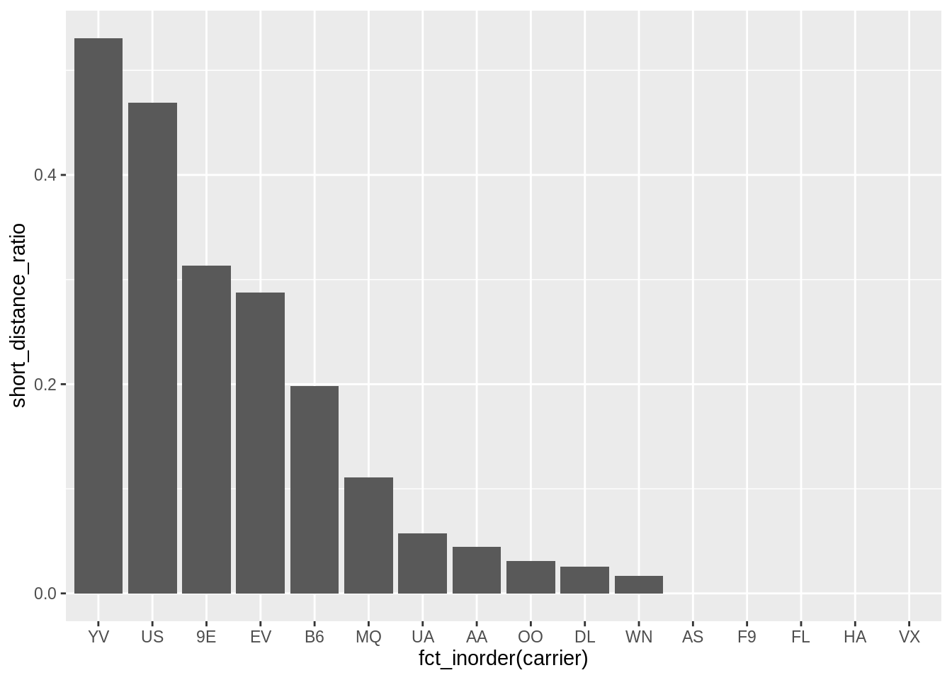
More exercises
Find more exercises in item 1 of Section 5.6.7 of r4ds.
Copyright © 2019 Kirill Müller. Licensed under CC BY-NC 4.0.