Summarize by multiple variables

Flights per day

How many flights flew out of NYC each day?

flights %>% 
  count(___, ___, ___)

► Solution:

flights %>% 
  count(year, month, day)

## # A tibble: 365 x 4
##     year month   day     n
##    <int> <int> <int> <int>
##  1  2013     1     1   842
##  2  2013     1     2   943
##  3  2013     1     3   914
##  4  2013     1     4   915
##  5  2013     1     5   720
##  6  2013     1     6   832
##  7  2013     1     7   933
##  8  2013     1     8   899
##  9  2013     1     9   902
## 10  2013     1    10   932
## # … with 355 more rows

Distinct airlines per relation

Which relation is serviced by the largest number of distinct airlines? Find a solution using summarize(), one using count(), and one using tally(). Which is more elegant?

flights %>%
  group_by(___, ___, airline) %>%
  summarize(n = n()) %>%
  summarize(n_airlines = ___) %>%
  ungroup() %>%
  arrange(___) %>%
  head(1)

flights %>%
  count(_____) %>%
  count(_____) %>%
  _____ %>%
  _____

flights %>%
  group_by(_____) %>%
  tally() %>%
  tally(wt = NULL) %>%
  _____ %>%
  _____

► Solution:

flights %>%
  group_by(origin, dest, carrier) %>%
  summarize(n_flights = n()) %>%
  summarize(n_distinct_carriers = n()) %>%
  ungroup() %>% 
  arrange(desc(n_distinct_carriers))

## # A tibble: 224 x 3
##    origin dest  n_distinct_carriers
##    <chr>  <chr>               <int>
##  1 EWR    DTW                     5
##  2 EWR    MSP                     5
##  3 JFK    LAX                     5
##  4 JFK    SFO                     5
##  5 JFK    TPA                     5
##  6 LGA    ATL                     5
##  7 LGA    CLE                     5
##  8 LGA    CLT                     5
##  9 EWR    ATL                     4
## 10 JFK    AUS                     4
## # … with 214 more rows

Much shorter:

flights %>%
  count(origin, dest, carrier) %>%
  count(origin, dest) %>% 
  ungroup() %>% 
  arrange(desc(n))

## # A tibble: 224 x 3
##    origin dest      n
##    <chr>  <chr> <int>
##  1 EWR    DTW       5
##  2 EWR    MSP       5
##  3 JFK    LAX       5
##  4 JFK    SFO       5
##  5 JFK    TPA       5
##  6 LGA    ATL       5
##  7 LGA    CLE       5
##  8 LGA    CLT       5
##  9 EWR    ATL       4
## 10 JFK    AUS       4
## # … with 214 more rows

Alternatively:

flights %>%
  group_by(origin, dest, carrier) %>%
  tally() %>%
  tally(wt = NULL) %>%
  ungroup() %>%
  arrange(desc(n))

## # A tibble: 224 x 3
##    origin dest      n
##    <chr>  <chr> <int>
##  1 EWR    DTW       5
##  2 EWR    MSP       5
##  3 JFK    LAX       5
##  4 JFK    SFO       5
##  5 JFK    TPA       5
##  6 LGA    ATL       5
##  7 LGA    CLE       5
##  8 LGA    CLT       5
##  9 EWR    ATL       4
## 10 JFK    AUS       4
## # … with 214 more rows

Cancelled flights per month per airline

Compute the share of cancelled flights per month per airline.

cancelled_flights <-
  flights %>% 
  group_by(_____) %>% 
  summarize(share_of_cancelled = _____) %>%
  ungroup()

cancelled_flights

► Solution:

cancelled_flights <-
  flights %>% 
  group_by(carrier, month) %>% 
  summarize(share_of_cancelled = mean(is.na(dep_time))) %>%
  ungroup()

cancelled_flights

## # A tibble: 185 x 3
##    carrier month share_of_cancelled
##    <chr>   <int>              <dbl>
##  1 9E          1             0.0477
##  2 9E          2             0.0727
##  3 9E          3             0.0695
##  4 9E          4             0.0688
##  5 9E          5             0.0506
##  6 9E          6             0.112 
##  7 9E          7             0.0870
##  8 9E          8             0.0536
##  9 9E          9             0.0409
## 10 9E         10             0.0185
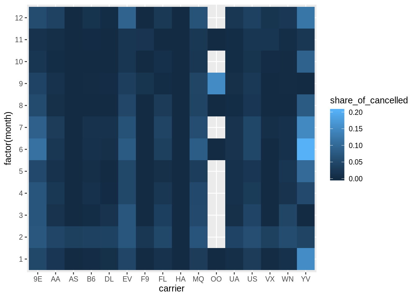
## # … with 175 more rows

Heat map of cancelled flights

Create a heat map of cancelled flights.

cancelled_flights <-
  _____

cancelled_flights %>% 
  ggplot() +
  geom_raster(
    aes(
      x = ___,
      y = factor(month),
      fill = ___
    )
  )

► Solution:

cancelled_flights %>%
  ggplot() +
  geom_raster(
    aes(
      x = carrier,
      y = factor(month),
      fill = share_of_cancelled
    )
  )

More exercises

Find more exercises in Section 5.6.7 of r4ds.

Summarize by multiple variables

Kirill Müller, cynkra GmbH

Flights per day

Distinct airlines per relation

Cancelled flights per month per airline

Heat map of cancelled flights

More exercises