Color, shape, alpha
Kirill Müller, Patrick Schratz
Map to the color aesthetic
In the hwy vs. displ plot, map an additional variable to the “color” aesthetic. Which cars consume more fuel than expected by the general trend?
ggplot(_____) +
  geom_point(mapping = aes(x = ___, y = ___, color = ___))
► Solution:
Simply insert color = <var> in the aes() call, where <var> is a variable in the mpg dataset:
ggplot(data = mpg) +
  geom_point(mapping = aes(x = displ, y = hwy, color = class))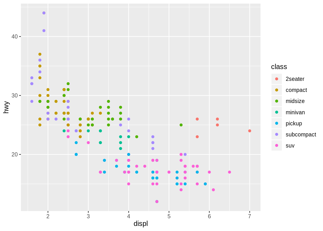
ggplot(data = mpg) +
  geom_point(mapping = aes(x = displ, y = hwy, color = cyl))
ggplot(data = mpg) +
  geom_point(mapping = aes(x = displ, y = hwy, color = trans))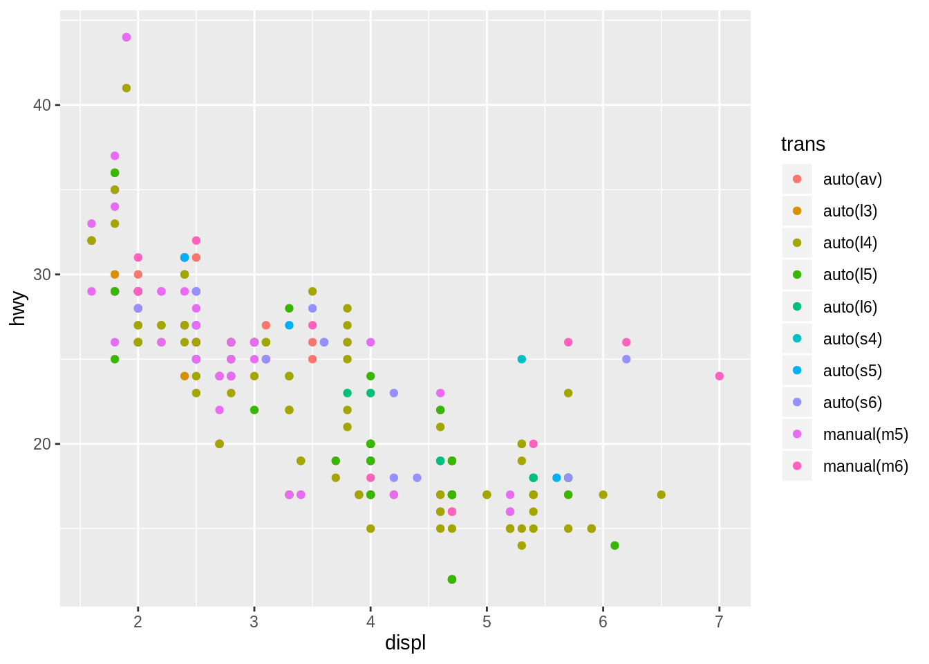
ggplot(data = mpg) +
  geom_point(mapping = aes(x = displ, y = hwy, color = drv))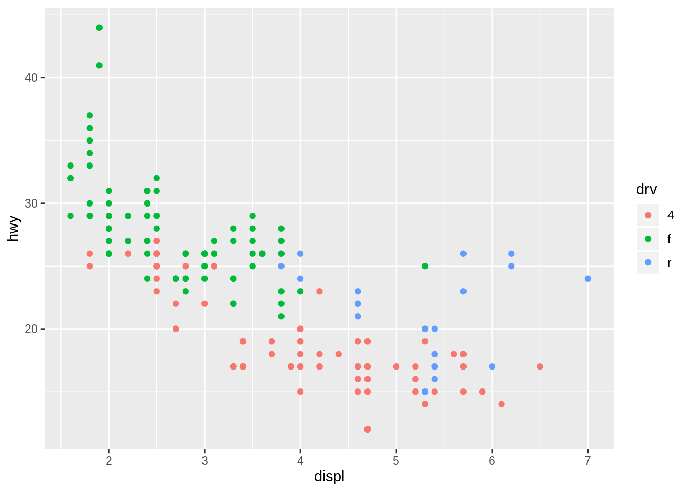
Map to other aesthetics
Experiment with the “color”, “shape”, “size”, and “alpha” aesthetics. Which combinations of attribute class (categorical/continuous) and aesthetics work well, which don’t? Expand on the more surprising examples in the previous exercises.
Hint: Use factor(year) to convert continuous variables with a limited set of values to categorical variables.
ggplot(_____) +
  geom_point(mapping = aes(x = ___, y = ___, ___ = ___))
► Solution:
Looks like the cars with large displacement are two-seaters with rear drivetrain.
The following won’t work, because cyl is stored as a continuous variable:
ggplot(data = mpg) +
  geom_point(mapping = aes(x = displ, y = hwy, shape = cyl))
## Error: A continuous variable can not be mapped to shape
The factor() function helps:
ggplot(data = mpg) +
  geom_point(mapping = aes(x = displ, y = hwy, shape = factor(cyl)))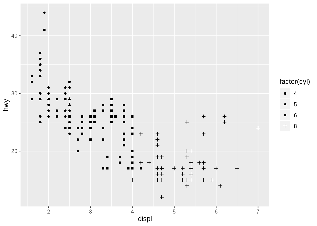
On the other hand, a continuous variable is fine for the “size” aesthetic…
ggplot(data = mpg) +
  geom_point(mapping = aes(x = displ, y = hwy, size = cyl))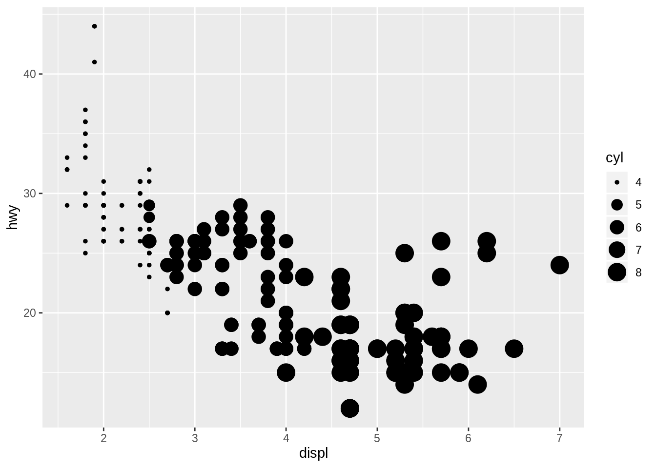
…which isn’t recommended (but still works) for a categorical variable:
ggplot(data = mpg) +
  geom_point(mapping = aes(x = displ, y = hwy, size = factor(cyl)))
## Warning: Using size for a discrete variable is not advised.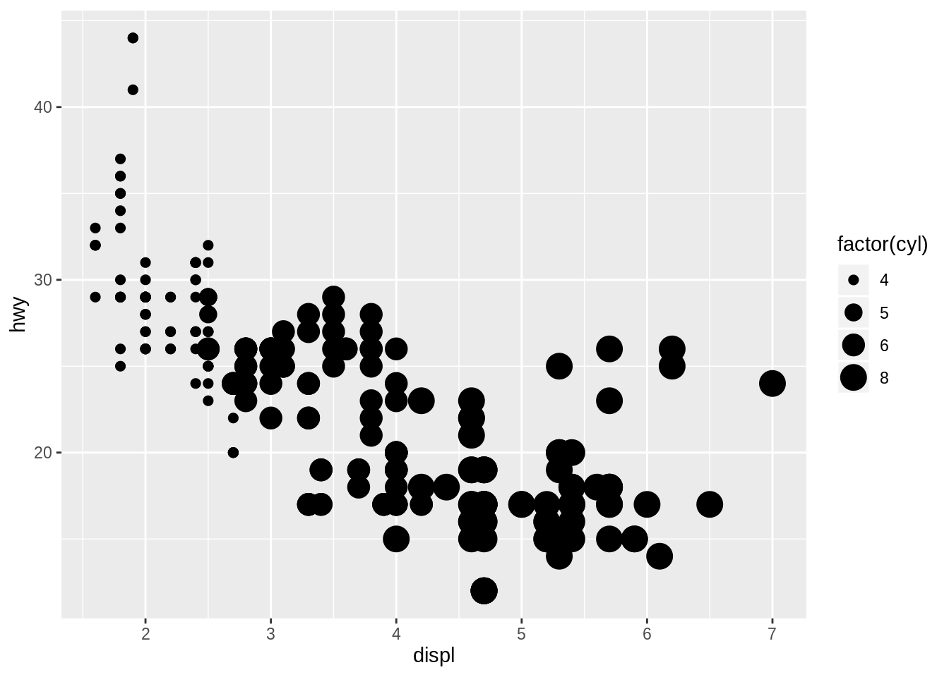
The “alpha” aesthetic controls transparency, and accepts both kinds of variable:
ggplot(data = mpg) +
  geom_point(mapping = aes(x = displ, y = hwy, alpha = cyl))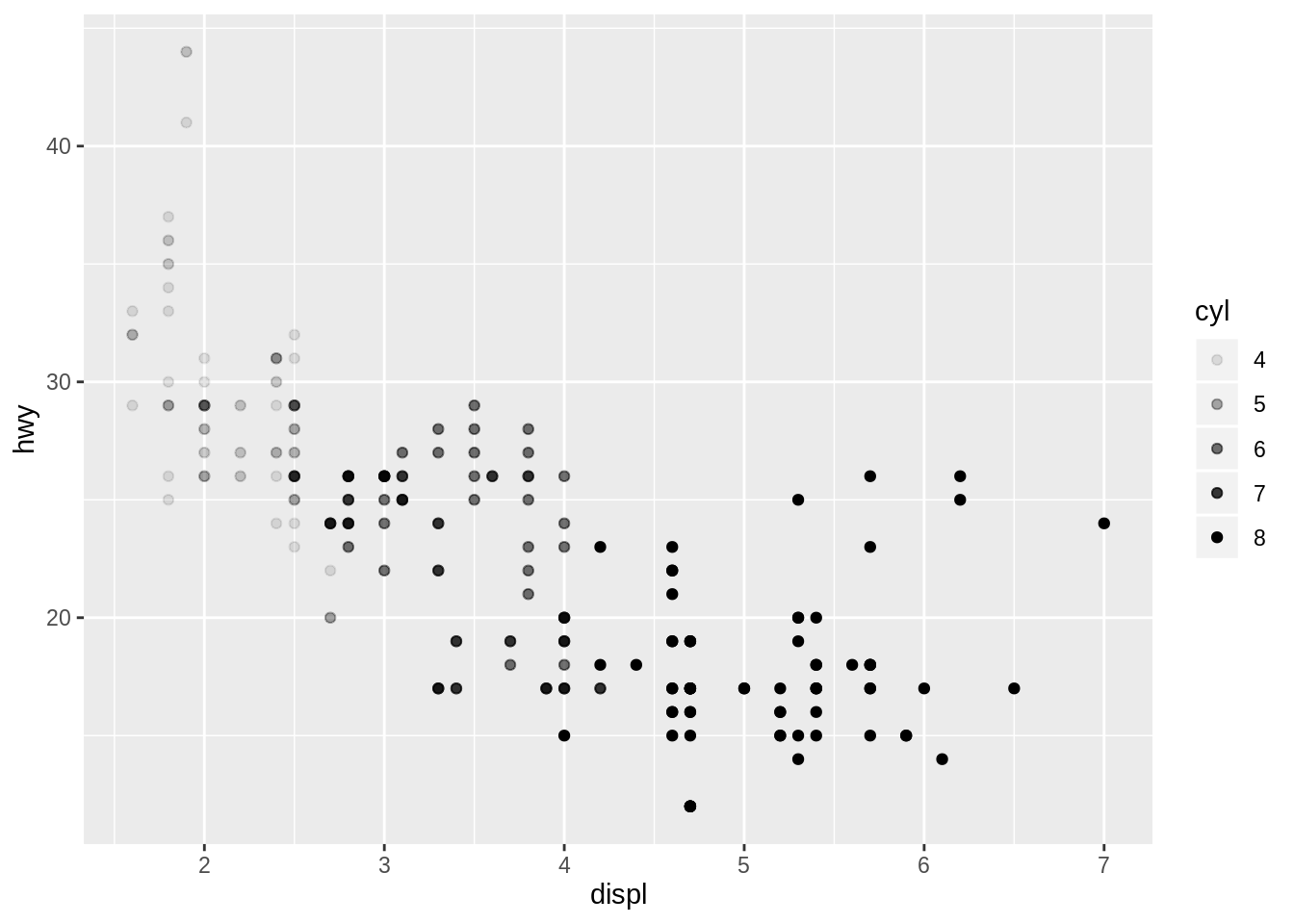
ggplot(data = mpg) +
  geom_point(mapping = aes(x = displ, y = hwy, alpha = factor(cyl)))
## Warning: Using alpha for a discrete variable is not advised.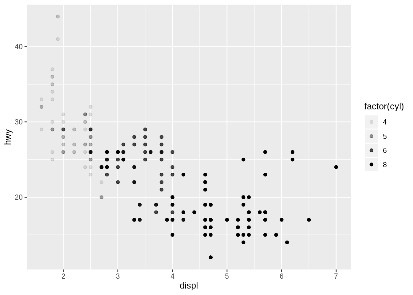
Change more than one aesthetic
Can you change both color and shape at the same time? What about the other aesthetics?
ggplot(_____) +
  geom_point(mapping = aes(x = ___, y = ___, ___ = ___, ___ = ___))
► Solution:
You can change any number of properties of a geom at your discretion, this is one of ggplot2’s strenghts.
ggplot(data = mpg) +
  geom_point(mapping = aes(
    x = displ,
    y = hwy,
    color = class,
    size = cyl,
    shape = drv,
    alpha = fl
  ))
## Warning: Using alpha for a discrete variable is not advised.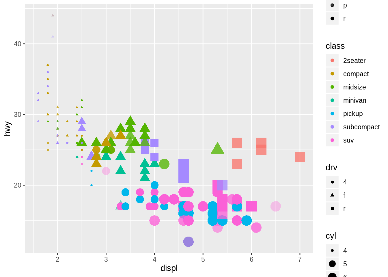
Map a variable to more than one aesthetic
What happens if you map the same variable to more than one aesthetic?
ggplot(_____) +
  geom_point(mapping = aes(x = ___, y = ___, ___ = ___, ___ = ___))
► Solution:
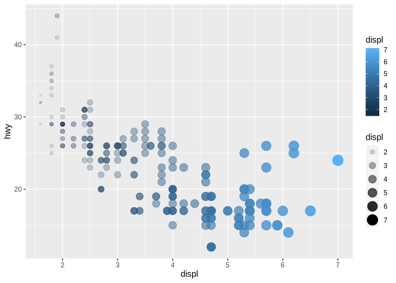
There are no restrictions on how many times a variable is mapped in any given plot:
ggplot(data = mpg) +
  geom_point(mapping = aes(
    x = displ,
    y = hwy,
    color = displ,
    size = displ,
    alpha = displ
  ))
More exercises
Find more exercises in Section 3.3.1 of r4ds.
Copyright © 2019 Kirill Müller. Licensed under CC BY-NC 4.0.