Mutate
Kirill Müller, cynkra GmbH
Speed as miles per hour
Store the speed for each flight as miles per hour in a new variable.
flights %>%
  mutate(miles_per_hour = air_time ___ distance ___ ___)
► Solution:
flights %>%
  mutate(miles_per_hour = distance / air_time * 60)
## # A tibble: 336,776 x 20
## year month day dep_time sched_dep_time dep_delay arr_time sched_arr_time
## <int> <int> <int> <int> <int> <dbl> <int> <int>
## 1 2013 1 1 517 515 2 830 819
## 2 2013 1 1 533 529 4 850 830
## 3 2013 1 1 542 540 2 923 850
## 4 2013 1 1 544 545 -1 1004 1022
## 5 2013 1 1 554 600 -6 812 837
## 6 2013 1 1 554 558 -4 740 728
## 7 2013 1 1 555 600 -5 913 854
## 8 2013 1 1 557 600 -3 709 723
## 9 2013 1 1 557 600 -3 838 846
## 10 2013 1 1 558 600 -2 753 745
## # … with 336,766 more rows, and 12 more variables: arr_delay <dbl>,
## # carrier <chr>, flight <int>, tailnum <chr>, origin <chr>, dest <chr>,
## # air_time <dbl>, distance <dbl>, hour <dbl>, minute <dbl>, time_hour <dttm>,
## # miles_per_hour <dbl>Speed as miles per minute
Can you use an intermediate variable to clarify the intent? How do you remove the intermediate variable?
flights %>%
  mutate(miles_per_minute = _____) %>%
  mutate(miles_per_hour = _____) %>%
  select(_____)
► Solution:
flights %>%
  mutate(miles_per_minute = distance / air_time) %>%
  mutate(miles_per_hour = miles_per_minute * 60) %>%
  select(-miles_per_minute)
## # A tibble: 336,776 x 20
## year month day dep_time sched_dep_time dep_delay arr_time sched_arr_time
## <int> <int> <int> <int> <int> <dbl> <int> <int>
## 1 2013 1 1 517 515 2 830 819
## 2 2013 1 1 533 529 4 850 830
## 3 2013 1 1 542 540 2 923 850
## 4 2013 1 1 544 545 -1 1004 1022
## 5 2013 1 1 554 600 -6 812 837
## 6 2013 1 1 554 558 -4 740 728
## 7 2013 1 1 555 600 -5 913 854
## 8 2013 1 1 557 600 -3 709 723
## 9 2013 1 1 557 600 -3 838 846
## 10 2013 1 1 558 600 -2 753 745
## # … with 336,766 more rows, and 12 more variables: arr_delay <dbl>,
## # carrier <chr>, flight <int>, tailnum <chr>, origin <chr>, dest <chr>,
## # air_time <dbl>, distance <dbl>, hour <dbl>, minute <dbl>, time_hour <dttm>,
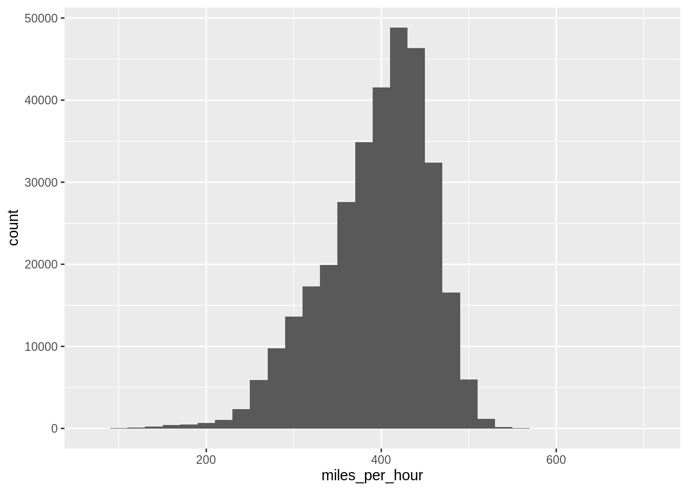
## # miles_per_hour <dbl>Speed, visualized
Visualize the speed distribution as a histogram. Would this visualization work without involving mutate()?
flights %>%
  ______ %>%
  ggplot(aes(___)) +
  _____

# Alternative:
flights %>%
  ggplot(aes(___)) +
  _____
► Solution:
flights %>%
  mutate(miles_per_hour = distance / air_time * 60) %>%
  ggplot() +
  geom_histogram(
    aes(miles_per_hour),
    na.rm = TRUE,
    binwidth = 20
  )
flights %>%
  ggplot() +
  geom_histogram(aes(distance / air_time))
## `stat_bin()` using `bins = 30`. Pick better value with `binwidth`.## Warning: Removed 9430 rows containing non-finite values (stat_bin).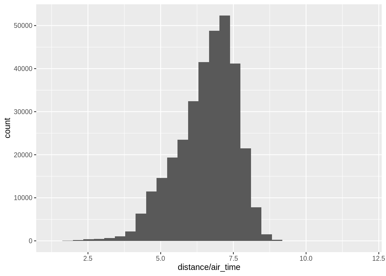
On time status
Create a new logical variable that indicates if the flight arrived on time.
flights %>%
  mutate(on_time = (_____))
► Solution:
flights %>%
  mutate(
    on_time = (arr_delay <= 0)
  )
## # A tibble: 336,776 x 20
## year month day dep_time sched_dep_time dep_delay arr_time sched_arr_time
## <int> <int> <int> <int> <int> <dbl> <int> <int>
## 1 2013 1 1 517 515 2 830 819
## 2 2013 1 1 533 529 4 850 830
## 3 2013 1 1 542 540 2 923 850
## 4 2013 1 1 544 545 -1 1004 1022
## 5 2013 1 1 554 600 -6 812 837
## 6 2013 1 1 554 558 -4 740 728
## 7 2013 1 1 555 600 -5 913 854
## 8 2013 1 1 557 600 -3 709 723
## 9 2013 1 1 557 600 -3 838 846
## 10 2013 1 1 558 600 -2 753 745
## # … with 336,766 more rows, and 12 more variables: arr_delay <dbl>,
## # carrier <chr>, flight <int>, tailnum <chr>, origin <chr>, dest <chr>,
## # air_time <dbl>, distance <dbl>, hour <dbl>, minute <dbl>, time_hour <dttm>,
## # on_time <lgl>On time status, visualized
Visualize the aggregated on-time status per airline with a useful text.
flights %>%
  flights %>%
  mutate(
    on_time = _____,
    on_time_desc = if_else(___, "On time", ___)
  ) %>%
  ggplot(aes(___)) +
  geom_bar()
► Solution:
flights %>%
  mutate(
    on_time = (arr_delay <= 0),
    on_time_desc = if_else(on_time, "On time", "Delayed")
  ) %>%
  ggplot(aes(x = carrier, fill = on_time_desc)) +
  geom_bar()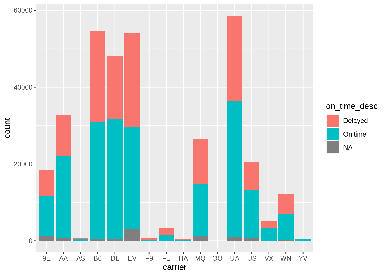
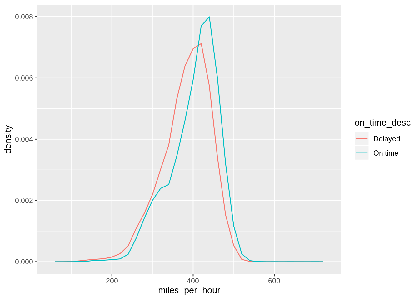
Speed distributions
Can you detect a difference in the speed distributions of on-time vs. delayed flights? Ose color of faceting.
speed_and_on_time_info <-
  _____

speed_and_on_time_info %>%
  ggplot() +
  geom_freqpoly(
    aes(x = ___, y = ..density.., color = ___),
    na.rm = TRUE,
    binwidth = 20
  )

speed_and_on_time_info %>%
  ggplot() +
  geom_histogram(
    aes(x = ___),
    na.rm = TRUE,
    binwidth = 20
  ) +
  facet_wrap(~___, ncol = 1)
► Solution:
speed_and_on_time_info <-
  flights %>%
  mutate(
    miles_per_minute = distance / air_time,
    miles_per_hour = miles_per_minute * 60
  ) %>%
  select(-miles_per_minute) %>%
  mutate(
    on_time = (arr_delay <= 0),
    on_time_desc = if_else(on_time, "On time", "Delayed")
  ) %>%
  select(-on_time)

speed_and_on_time_info %>%
  ggplot() +
  geom_freqpoly(
    aes(x = miles_per_hour, y = ..density.., color = on_time_desc),
    na.rm = TRUE,
    binwidth = 20
  )
speed_and_on_time_info %>%
  filter(!is.na(on_time_desc)) %>%
  ggplot() +
  geom_histogram(
    aes(x = miles_per_hour),
    na.rm = TRUE,
    binwidth = 20
  ) +
  facet_wrap(~on_time_desc, ncol = 1)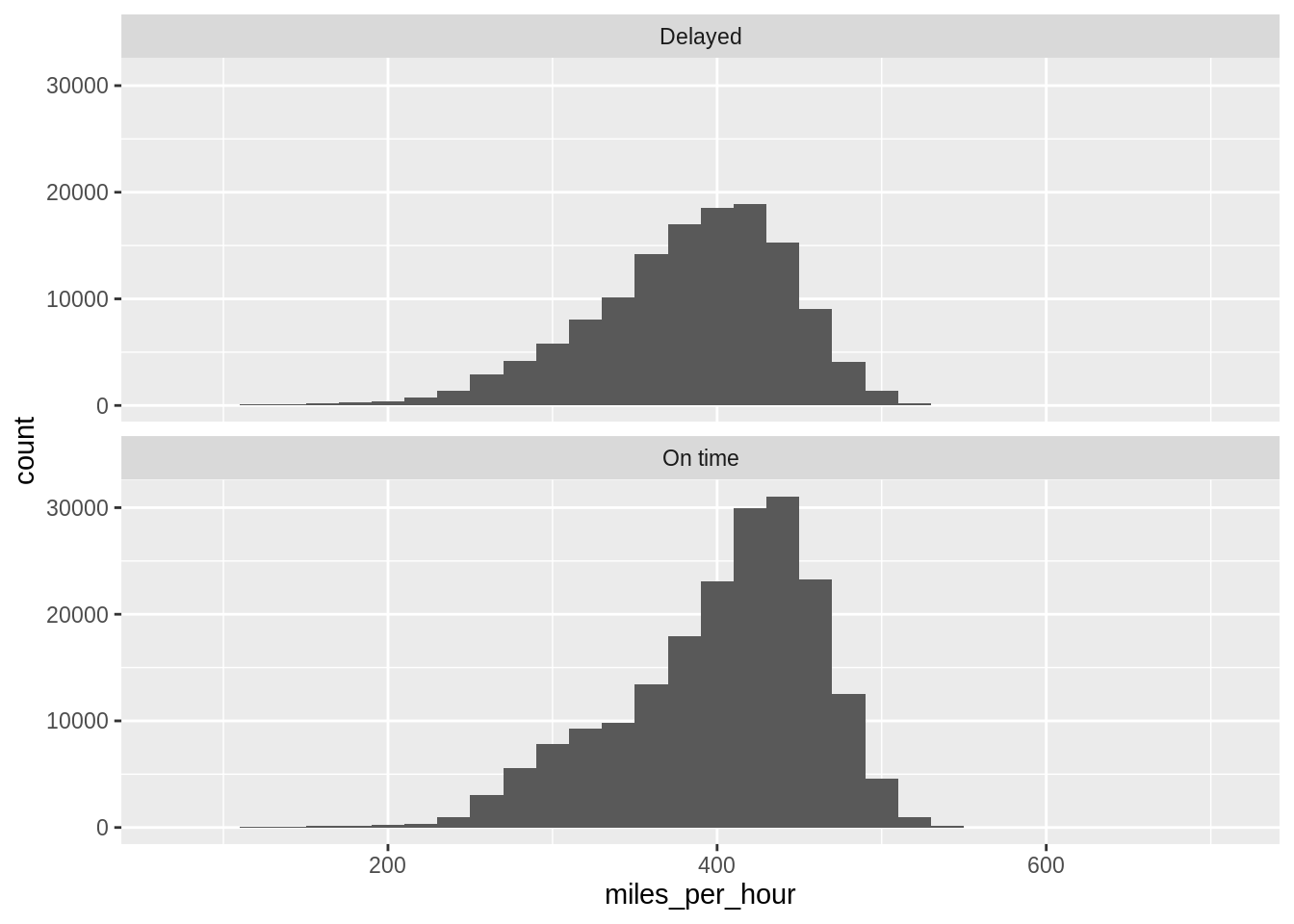
Date
Create two new variables date_hour and date_ymd, using as.Date() or lubridate::make_date(), respectively. Are the two values the same for all observations? What happens if we omit the tz argument to as.Date()?
flights %>%
  mutate(
    ___ = as.Date(___, tz = "EST"),
    ___ = lubridate::make_date(_____)
  ) %>%
  filter(___)
► Solution:
flights %>%
  mutate(
    date_hour = as.Date(time_hour, tz = "EST"),
    date_ymd = lubridate::make_date(year, month, day)
  ) %>%
  filter(date_hour != date_ymd)
## # A tibble: 0 x 21
## # … with 21 variables: year <int>, month <int>, day <int>, dep_time <int>,
## # sched_dep_time <int>, dep_delay <dbl>, arr_time <int>,
## # sched_arr_time <int>, arr_delay <dbl>, carrier <chr>, flight <int>,
## # tailnum <chr>, origin <chr>, dest <chr>, air_time <dbl>, distance <dbl>,
## # hour <dbl>, minute <dbl>, time_hour <dttm>, date_hour <date>,
## # date_ymd <date>Deviation from average departure delay
Visualize the deviation from the overall average departure delay for the three airports of New York City. Consider using a violin plot.
flights %>%
  mutate(dep_delay_dev = ___ - mean(___)) %>%
  ggplot(aes(___)) +
  _____ +
  _____
► Solution:
flights %>%
  mutate(dev = dep_delay - mean(dep_delay, na.rm = TRUE)) %>%
  ggplot() +
  geom_violin(aes(x = origin, y = dev), na.rm = TRUE)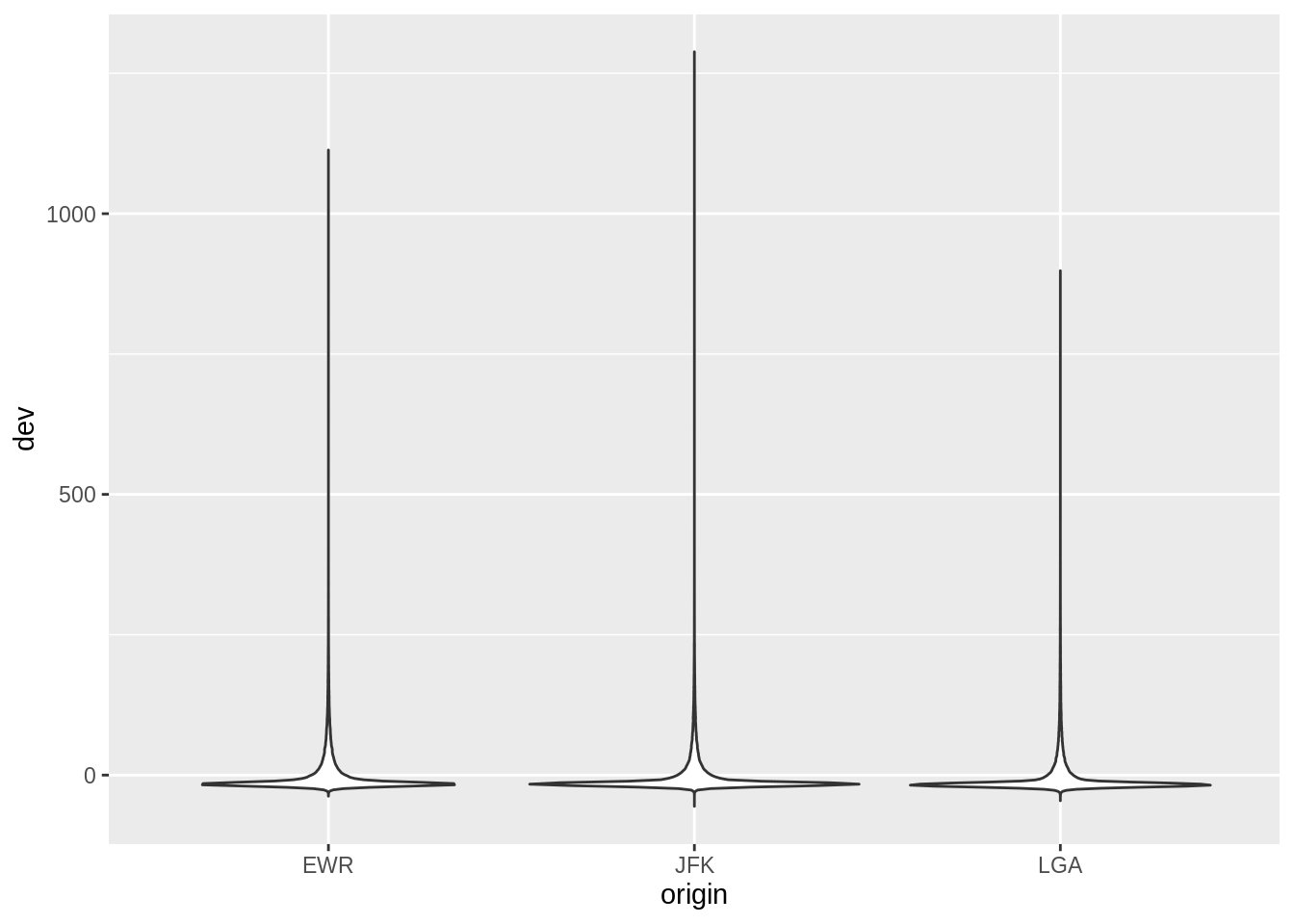
More exercises
Find more exercises in Section 5.5.2 of r4ds.
Copyright © 2019 Kirill Müller. Licensed under CC BY-NC 4.0.