Theming
Kirill Müller, cynkra GmbH
June 1, 2017
Favorite theme
Choose your favorite among the predefined themes.
Hint: All start with theme_...(), but watch out for theme_set().
► Solution:
For presentations, theme_bw() or theme_minimal() look useful:
ggplot(data = mpg) +
  theme_bw() +
  geom_jitter(mapping = aes(x = displ, y = hwy, color = class)) +
  scale_x_continuous(name = "Displacement") +
  scale_y_continuous(name = "Fuel economy [miles per gallon]") +
  scale_color_brewer(name = "Car class", palette = "Set2")
ggplot(data = mpg) +
  theme_minimal() +
  geom_jitter(mapping = aes(x = displ, y = hwy, color = class)) +
  scale_x_continuous(name = "Displacement") +
  scale_y_continuous(name = "Fuel economy [miles per gallon]") +
  scale_color_brewer(name = "Car class", palette = "Set2")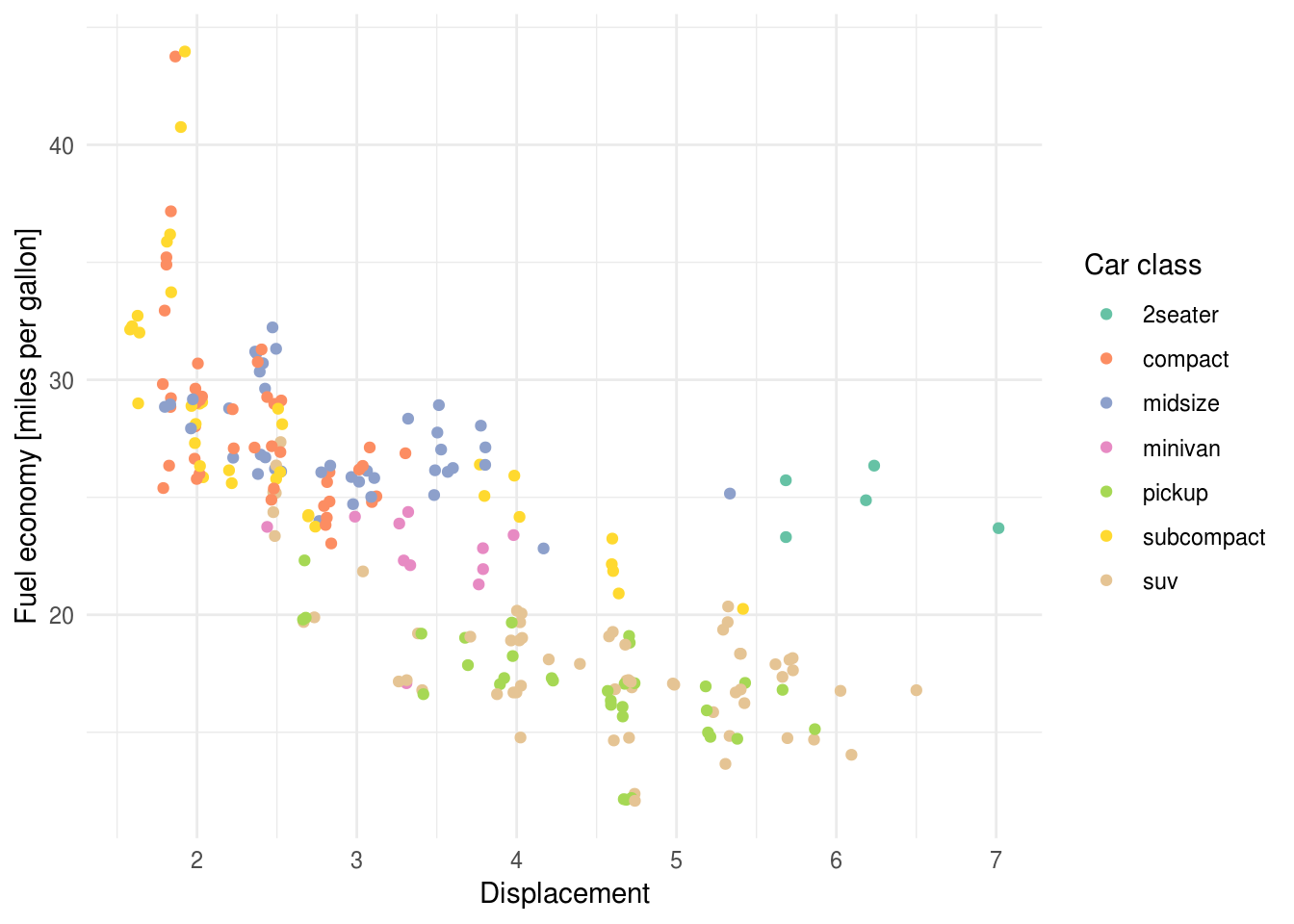
Legend at bottom
Apply theme(legend.position = "bottom") to a plot with a color or fill legend. What happens if you then apply theme_bw()? Why?
► Solution:
ggplot(data = mpg) +
  theme_bw() +
  geom_jitter(mapping = aes(x = displ, y = hwy, color = class)) +
  scale_x_continuous(name = "Displacement") +
  scale_y_continuous(name = "Fuel economy [miles per gallon]") +
  scale_color_brewer(name = "Car class", palette = "Set2") +
  theme(legend.position = "bottom")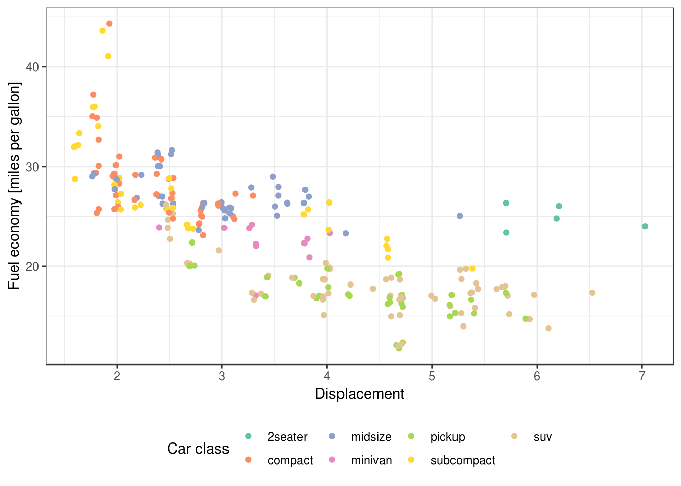
theme_bw() overwrites everything, including the legend position:
ggplot(data = mpg) +
  geom_jitter(mapping = aes(x = displ, y = hwy, color = class)) +
  scale_x_continuous(name = "Displacement") +
  scale_y_continuous(name = "Fuel economy [miles per gallon]") +
  scale_color_brewer(name = "Car class", palette = "Set2") +
  theme(legend.position = "bottom") +
  theme_bw()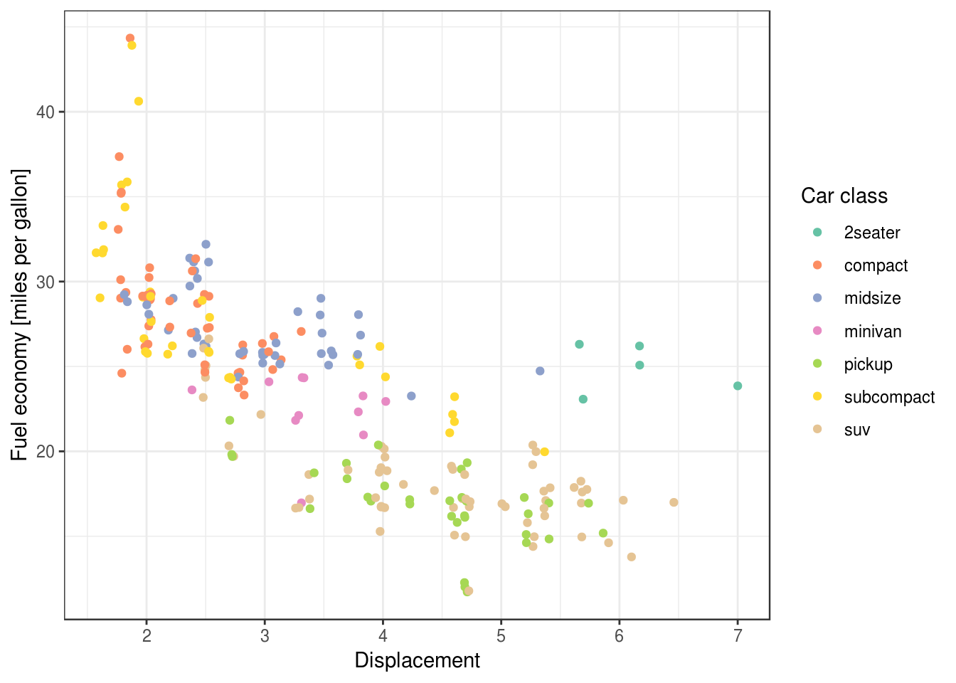
Copyright © 2018 Kirill Müller. Licensed under CC BY-NC 4.0.